import numpy as np
import matplotlib.pyplot as plt
from sklearn.preprocessing import PolynomialFeatures
from sklearn.linear_model import LinearRegression
from sklearn.metrics import mean_squared_error
np.random.seed(0)
X = 2 - 3 * np.random.normal(0, 1, 100)
y = X - 2 * (X ** 2) + np.random.normal(-3, 3, 100)
X = X[:, np.newaxis]
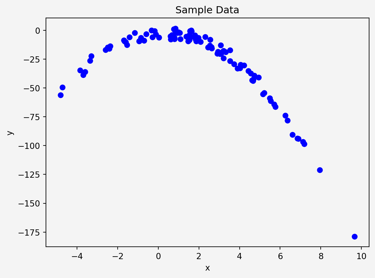
plt.scatter(X, y, color='blue')
plt.title("Sample Data")
plt.xlabel('x')
plt.ylabel('y')
plt.gca().set_facecolor('#f4f4f4')
plt.gcf().patch.set_facecolor('#f4f4f4')
plt.show()Polynomial Regression
Introduction
Polynomial regression is an extension of linear regression that captures the relationship between the dependent and independent variables by fitting a polynomial equation. Unlike linear regression, where the model assumes a straight-line relationship, polynomial regression allows for more complex relationships, enabling the model to fit non-linear data more accurately.
What is Polynomial Regression?
Polynomial regression is a type of regression where the relationship between the independent variable \(X\) and the dependent variable \(y\) is modeled as an \(n\)th degree polynomial. The general form of a polynomial regression model is:
\[ y = \beta_0 + \beta_1 X + \beta_2 X^2 + \beta_3 X^3 + \dots + \beta_n X^n + \epsilon \]
Where:
- \(y\) is the predicted output (dependent variable),
- \(X\) is the input feature (independent variable),
- \(\beta_0, \beta_1, \dots, \beta_n\) are the coefficients to be learned,
- \(\epsilon\) is the error term (the difference between the actual and predicted values),
- \(n\) is the degree of the polynomial.
Polynomial regression can model non-linear data by introducing polynomial terms (such as \(X^2, X^3\), etc.), but the model is still linear in terms of the coefficients, which is why it is often treated as a type of linear regression.
Mathematical Derivation of Polynomial Regression
The objective of polynomial regression, like linear regression, is to minimize the sum of squared errors (SSE) between the observed values \(y_i\) and the predicted values \(\hat{y}_i\). This can be done by applying the ordinary least squares (OLS) method.
For simplicity, let’s assume a second-degree polynomial regression model:
\[ \hat{y} = \beta_0 + \beta_1 X + \beta_2 X^2 \]
The error for each data point is the difference between the actual value \(y_i\) and the predicted value \(\hat{y}_i\):
\[ e_i = y_i - \hat{y}_i = y_i - (\beta_0 + \beta_1 X_i + \beta_2 X_i^2) \]
We aim to minimize the sum of squared errors (SSE):
\[ SSE = \sum_{i=1}^{m} (y_i - \hat{y}_i)^2 = \sum_{i=1}^{m} (y_i - (\beta_0 + \beta_1 X_i + \beta_2 X_i^2))^2 \]
Where \(m\) is the number of data points.
We can represent this problem in matrix form to generalize for higher-degree polynomials and simplify the calculation:
Let \(X\) represent the design matrix, where each column corresponds to a power of the independent variable \(X\):
\[ X = \begin{bmatrix} 1 & X_1 & X_1^2 \\ 1 & X_2 & X_2^2 \\ \vdots & \vdots & \vdots \\ 1 & X_m & X_m^2 \end{bmatrix} \]
Let \(\beta\) be the coefficient vector:
\[ \beta = \begin{bmatrix} \beta_0 \\ \beta_1 \\ \beta_2 \end{bmatrix} \]
And \(y\) be the output vector:
\[ y = \begin{bmatrix} y_1 \\ y_2 \\ \vdots \\ y_m \end{bmatrix} \]
The predicted values can be written as:
\[ \hat{y} = X \beta \]
To find the optimal coefficients \(\beta\), we minimize the SSE, which can be rewritten in matrix form as:
\[ SSE = (y - X\beta)^T(y - X\beta) \]
To minimize this, we take the derivative of the SSE with respect to \(\beta\) and set it to zero:
\[ \frac{\partial}{\partial \beta} (y - X\beta)^T(y - X\beta) = -2X^T(y - X\beta) = 0 \]
Solving for \(\beta\):
\[ \beta = (X^T X)^{-1} X^T y \]
This gives the optimal solution for the coefficients \(\beta\), which can be used to predict the output \(\hat{y}\). The detail proof of this parameter \(\hat{\beta}\) can be found in the multiple linear regression page.
Python Implementation of Polynomial Regression (One Variable)
We use PolynomialFeatures from Scikit-learn to transform our input data \(X\) to include polynomial terms (e.g., \(X^2, X^3\), etc.).
poly = PolynomialFeatures(degree=2, interaction_only=False, include_bias=True)
X_poly = poly.fit_transform(X)
Now we fit a linear regression model on the transformed polynomial features.
model = LinearRegression()
model.fit(X_poly, y)

y_pred = model.predict(X_poly)

print(f"Coefficients: {model.coef_}")
print(f"Intercept: {model.intercept_}")
print(f"Mean Squared Error: {mean_squared_error(y, y_pred)}")
Coefficients: [ 0. 0.96597113 -2.02225052]
Intercept: -2.4148356673536284
Mean Squared Error: 9.447441952450275Finally, let’s plot the polynomial curve that fits the data.
import operator
sort_axis = operator.itemgetter(0)
sorted_zip = sorted(zip(X, y_pred), key=sort_axis)
X_sorted, y_pred_sorted = zip(*sorted_zip)

# Plot the polynomial curve
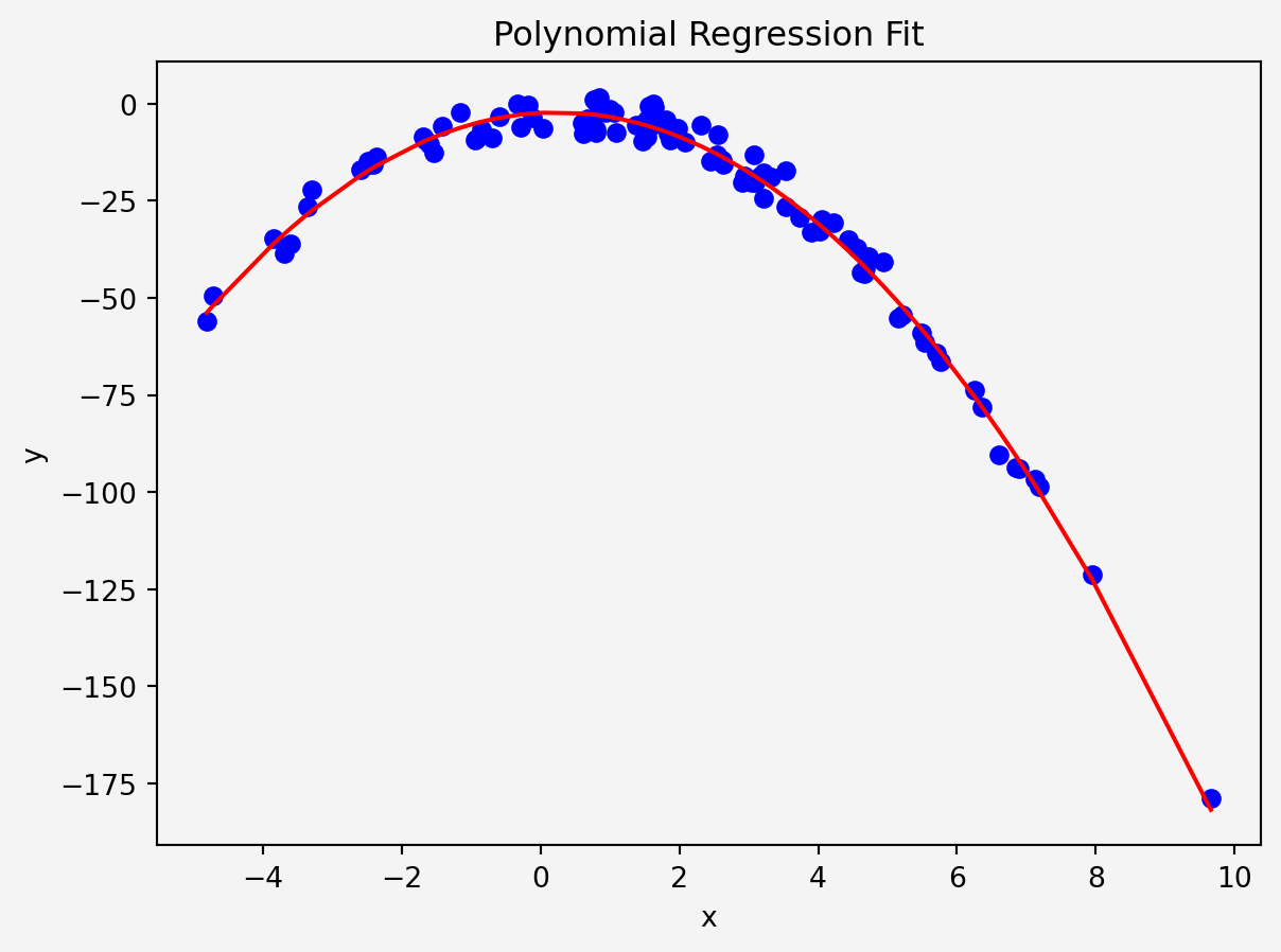
plt.scatter(X, y, color='blue')
plt.plot(X_sorted, y_pred_sorted, color='red')
plt.xlabel('x')
plt.ylabel('y')
plt.title("Polynomial Regression Fit")
plt.gca().set_facecolor('#f4f4f4')
plt.gcf().patch.set_facecolor('#f4f4f4')
plt.show()
We can evaluate the performance of the model by comparing the mean squared error (MSE) between the actual and predicted values:
mse = mean_squared_error(y, y_pred)
print(f"Mean Squared Error: {mse}")
Mean Squared Error: 9.447441952450275Python Implementation of Polynomial Regression (Two Variables)
We’ll generate some non-linear data and try to fit a polynomial regression model to it.
import pandas as pd
import seaborn as sns
from pandas.plotting import scatter_matrix
np.random.seed(0)
x1 = 2 - 3 * np.random.normal(0, 1, 100)
x2 = 4*np.random.normal(-2,2,100)
y = 2+3*x1 -4*x1**2 + 2 * x2 + np.random.normal(-3, 3, 100)
df={
    'x1':x1,
    'x2':x2,
    'y':y
}
df = pd.DataFrame(df)
print(df.head())
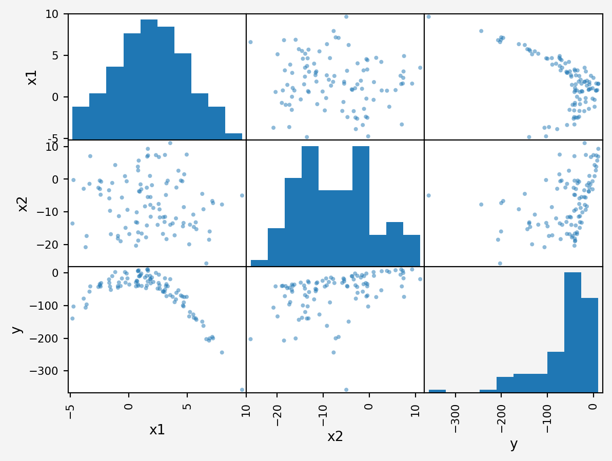
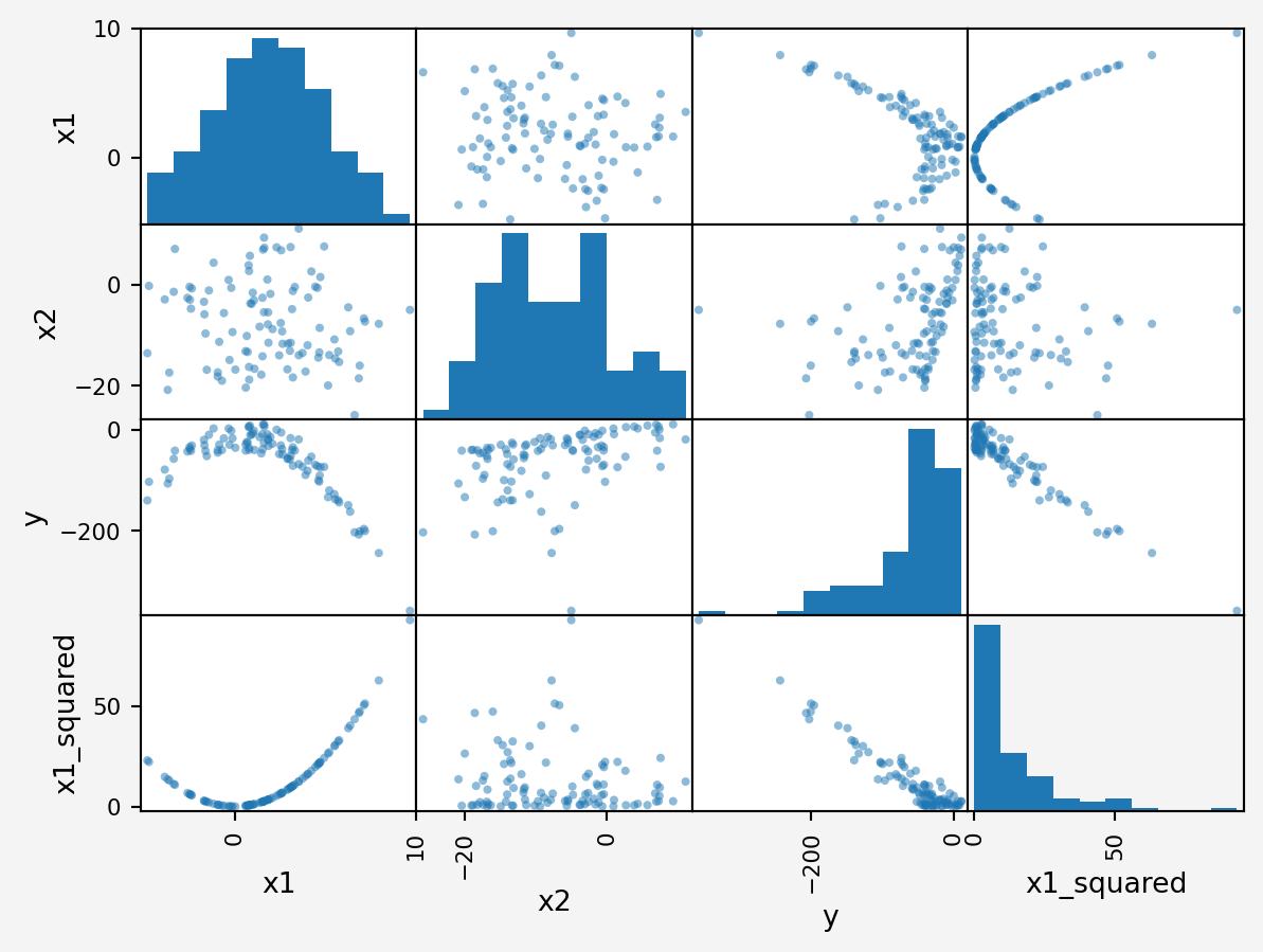
scatter_matrix(df)
plt.gca().set_facecolor('#f4f4f4')
plt.gcf().patch.set_facecolor('#f4f4f4')
plt.show()
x1 x2 y
0 -3.292157 7.065206 -41.206797
1 0.799528 -18.782072 -39.440680
2 -0.936214 -18.163880 -40.343409
3 -4.722680 -0.244826 -102.906711
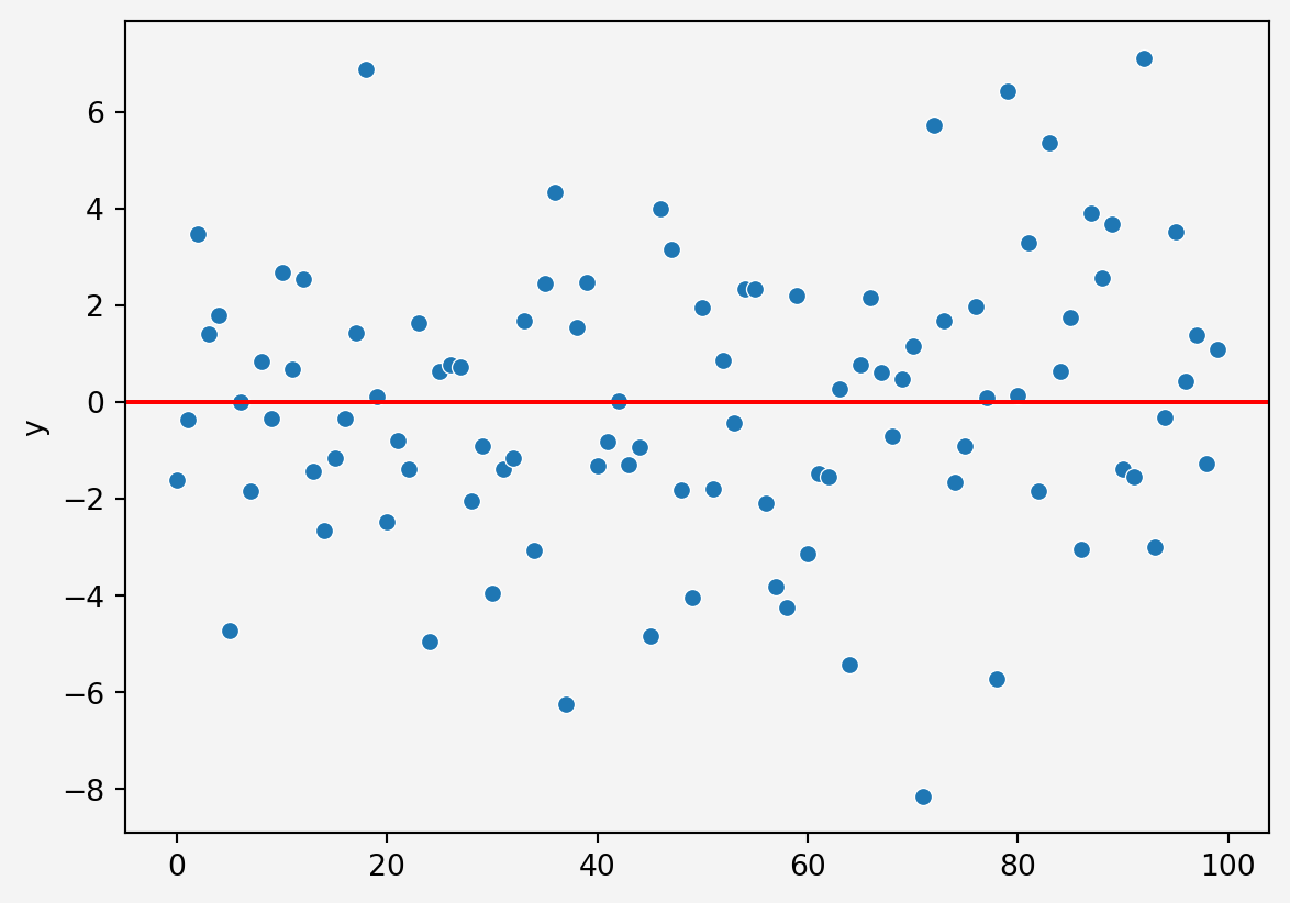
4 -3.602674 -17.384987 -96.574641Since it’s clear that the relationships are not linear. So if we fit a linear regression model, it won’t be a good fit.
X = df.drop('y', axis=1)
y = df.y
model1 = LinearRegression()
model1.fit(X,y)
pred1 = model1.predict(X)
residual1 = y - pred1
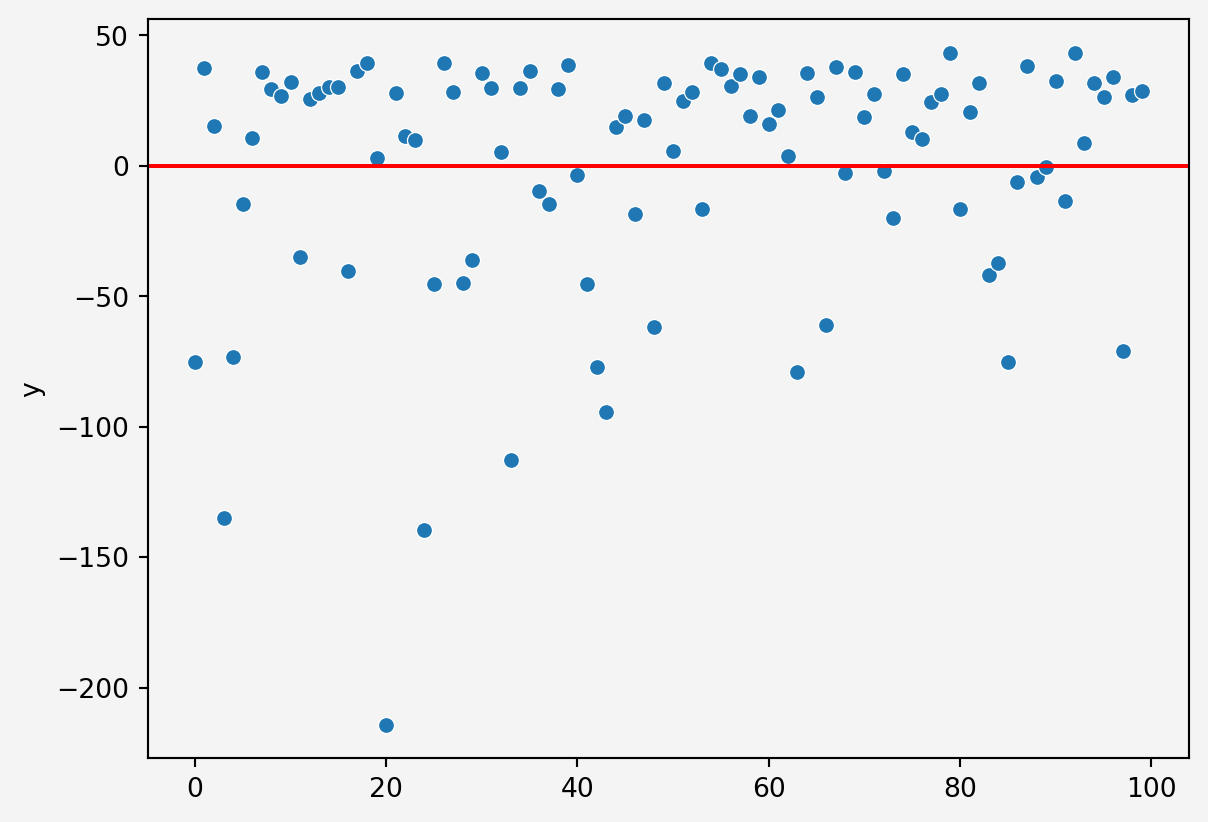
sns.scatterplot(residual1)
plt.axhline(y=0, c='r')
plt.gca().set_facecolor('#f4f4f4')
plt.gcf().patch.set_facecolor('#f4f4f4')
plt.show()
Therefore, we generate some non linear features from the given data.
df['x1_squared']=df.x1**2
scatter_matrix(df)
plt.gca().set_facecolor('#f4f4f4')
plt.gcf().patch.set_facecolor('#f4f4f4')
plt.show()
From this plot, we see that \(x1\) is parabolic and \(x2\) is linear in relationship with \(y\). So, how about a model that combines a linear and quadratic model?
X = df.drop('y', axis=1)
y = df.y
model2 = LinearRegression()
model2.fit(X,y)
pred2 = model2.predict(X)
residual2 = y - pred2
sns.scatterplot(residual2)
plt.axhline(y=0, c='r')
plt.gca().set_facecolor('#f4f4f4')
plt.gcf().patch.set_facecolor('#f4f4f4')
plt.show()
This one is much better.
Polynomial regression is a powerful technique that extends the basic linear regression model to capture non-linear relationships between variables. By transforming the input data into polynomial terms, the model becomes more flexible, allowing it to better fit data that doesn’t follow a linear pattern.
The mathematical derivation shows that polynomial regression is still linear in terms of its parameters, allowing us to use simple optimization techniques like ordinary least squares (OLS) for parameter estimation.
In Python, using Scikit-learn makes it easy to implement polynomial regression. We can increase the degree of the polynomial to improve model accuracy, but we need to be careful of overfitting, where the model becomes too complex and fits the noise in the data rather than the underlying pattern.
You may also like
Citation
@online{islam2024,
  author = {Islam, Rafiq},
  title = {Polynomial {Regression}},
  date = {2024-09-20},
  url = {https://mrislambd.github.io/dsandml/polyreg/},
  langid = {en}
}
