Bayesian Probabilistic Models for Classification
Introduction
Bayesian inference is a powerful statistical method that applies the principles of Bayes’s theorem to update the probability of a hypothesis as more evidence or information becomes available. It is widely used in various fields including machine learning, to make predictions and decisions under uncertainty.
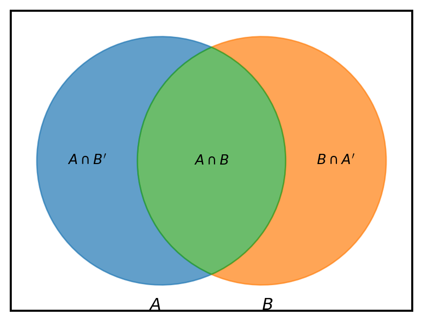
Bayes’s theorem is based on the definition of conditional probability. For two events \(A\) and \(B\) with \(\mathbb{P}(B) \neq 0\), we define the conditional probability of occurring \(A\) given that \(B\) has already occurred.
\(\mathbb{P}(A|B)=\frac{\mathbb{P}(A\cap B)}{\mathbb{P}(B)}\)
Similarly, the conditional probability of occuring \(B\) given that \(A\) has already occured with \(\mathbb{P}(A) \ne 0\) is
\[
\mathbb{P}(B|A)=\frac{\mathbb{P}(A\cap B)}{\mathbb{P}(A)}
\]
From this equation, we can derive that the joint probability of \(A\cap B\) is \[ \mathbb{P}(A\cap B) = \mathbb{P}(B | A) \mathbb{P} (A) = \mathbb{P}(A | B) \mathbb{P} (B) \]
Bayes’s Theorem
For Two Events or Random Variables
Bayes’s theorem is based on these conditional probabilities. It states that the likelihood of occuring the event \(A\) given that the event \(B\) has occured is given as
\[ \mathbb{P}(A | B) = \frac{\mathbb{P}(B | A)\mathbb{P}(A)}{\mathbb{P}(B)} = \frac{\mathbb{P}(B | A)\mathbb{P}(A)}{\mathbb{P}(B\cap A)+\mathbb{P}(B\cap A^c)} = \frac{\mathbb{P}(B | A)\mathbb{P}(A)}{\mathbb{P}(B | A)\mathbb{P}(A)+\mathbb{P}(A | B)\mathbb{P}(B)} \]
where, in Bayesin terminology,
- \(\mathbb{P}(A|B)\) is called posterior probability of \(A\) given the event \(B\) or simply, posterior distribution.
- \(\mathbb{P}(B|A)\) is the likelihood: the probability of evidence \(B\) given that \(A\) is true.
- \(\mathbb{P}(A)\) or \(\mathbb{P}(B)\) are the probabilities of occuring \(A\) and \(B\) respectively, without any dependence on each other.
- \(\mathbb{P}(A)\) is called the prior probability or prior distribution and \(\mathbb{P}(B)\) is called the marginal likelihood or marginal probabilities.
For two continuous random variable \(X\) and \(Y\), the conditional probability density function of \(X\) given the occurence of the value \(y\) of \(Y\) can be given as
\[ f_{X|Y} (x | y) =\frac{f_{X,Y}(x,y)}{f_Y(y)} \]
or the otherway around,
\[
f_{Y|X} (y | x) =\frac{f_{X,Y}(x,y)}{f_X(x)}
\]
Therefore, the continuous version of Bayes’s theorem is given as follows
\[ f_{Y|X}(y) = \frac{f_{X|Y}(x)f_Y(y)}{f_X(x)} \]
Generalization of Bayes’s Theorem
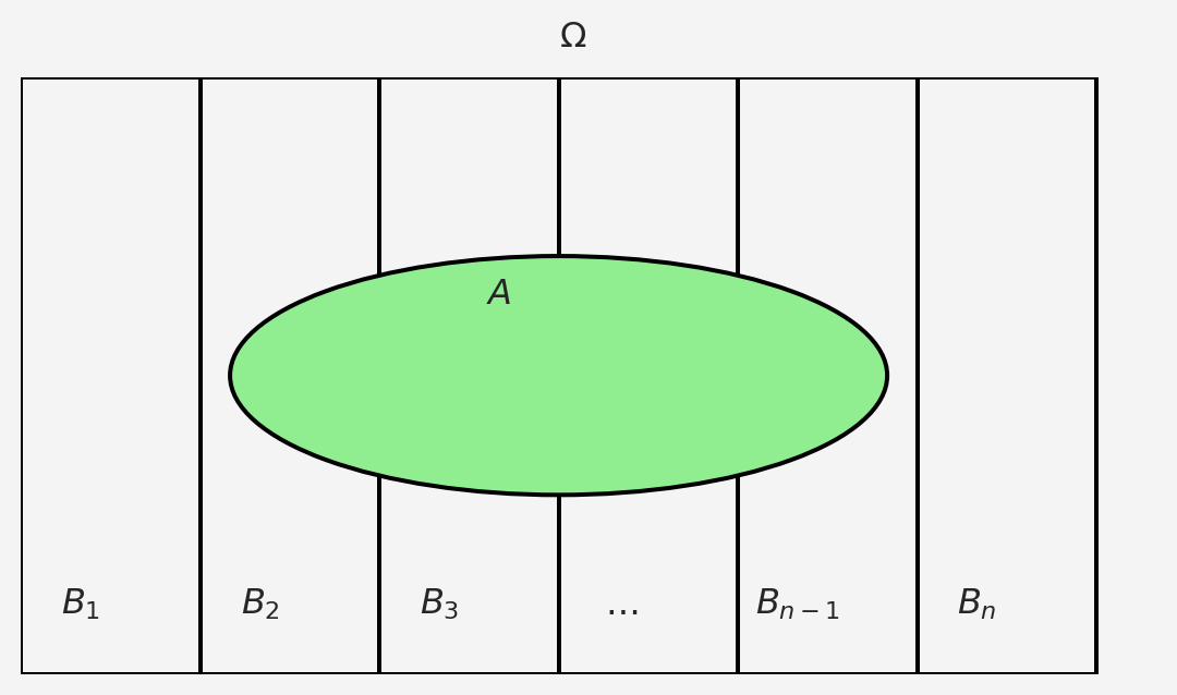
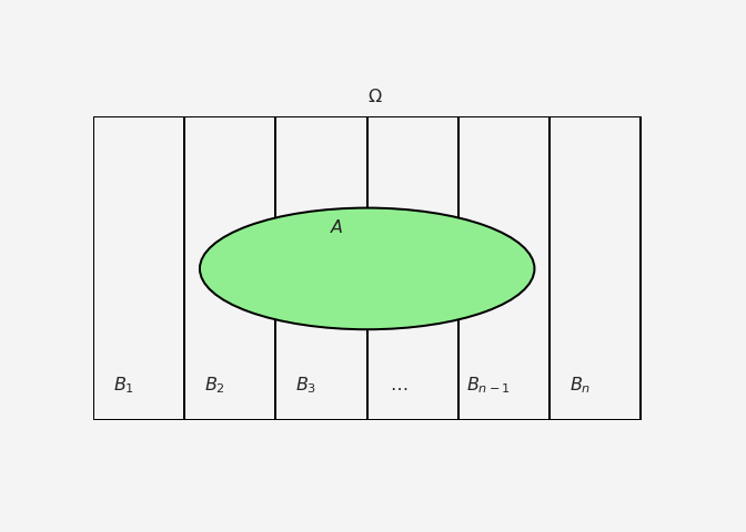
For \(n\) disjoint set of discrete events \(B_1,B_2\dots, B_n\) where \(\Omega = \cup_{i}^{n}B_i\) and for any event \(A\in \Omega\), we will have
\[
\mathbb{P}(A) = \sum_{i=1}^{n}\mathbb{P}(A\cap B_i)
\]
and this is true by the law of total probability.
Then the Bayes’s rule extends to the following
\[ \mathbb{P}(B_i|A) = \frac{\mathbb{P}(A|B_i)\mathbb{P}(B_i)}{\mathbb{P}(A)}=\frac{\mathbb{P}(A|B_i)\mathbb{P}(B_i)}{\sum_{i=1}^{n}\mathbb{P}(A|B_i)\mathbb{P}(B_i)} \]
The continuous version would be \[ f_{Y=y|X=x}(y|x) = \frac{f_{X|Y=y}(x)f_Y(y)}{\sum_{i=1}^{n}\int_{-\infty}^{\infty}f_{X|Y=y}(x|u)f_{Y}(u)du} \]
Probabilistic Models
Bayes’s theorem gets us the posterior probability given the data with a prior. Therefore, for classification tasks in machine learning, we can use Bayesin style models for classification by maximizing the numerator and minimizing the denominator in the previous equation, for any given class. For instance, say we have a \(d-\) dimensional data collected as a random matrix \(X\) and the response variable \(y\) is a categorical one with \(c\) categories. Then for a given data vector \(X'\), the posterior distibution that it falls for category \(j\) is given as
\[ \mathbb{P}(y=j|X=X')=\frac{\pi_j f_j(X')}{\sum_{i=1}^{c}\pi_i f_i(X')} \]
where,
- \(f_i(X)\) is the probability density function of the features conditioned on \(y\) being class \(i\)
- \(\pi_i =\mathbb{P}(y=i)\)
We can estimate \(\pi_i\) as the fraction of observations which belong to class \(i\).
Linear Discriminant Analysis (LDA)
To connect Linear Discriminant Analysis (LDA) with the Bayesian probabilistic classification, we start by considering the Bayes Theorem and the assumptions made in LDA. We adapt the Bayes theorem for classification as follows
\[ P(C_k | \mathbf{x}) = \frac{P(\mathbf{x} | C_k) P(C_k)}{P(\mathbf{x})} \]
Where:
- \(P(C_k | \mathbf{x})\) is the posterior probability that \(\mathbf{x}\) belongs to class \(C_k\),
- \(P(\mathbf{x} | C_k)\) is the likelihood (the probability of observing \(\mathbf{x}\) given class \(C_k\)),
- \(P(C_k)\) is the prior probability of class \(C_k\),
- \(P(\mathbf{x})\) is the marginal likelihood (normalizing constant).
Gaussian Assumption in LDA
LDA assumes that:
- The likelihood for each class follows a Gaussian distribution with a common covariance matrix \(\Sigma\), i.e.,
\[ P(\mathbf{x} | C_k) = \frac{1}{(2\pi)^{d/2} |\Sigma|^{1/2}} \exp\left(-\frac{1}{2} (\mathbf{x} - \boldsymbol{\mu}_k)^T \Sigma^{-1} (\mathbf{x} - \boldsymbol{\mu}_k)\right) \]
where \(\boldsymbol{\mu}_k\) is the mean of class \(C_k\) and \(\Sigma\) is the shared covariance matrix. Now let’s talk about \(\boldsymbol{\mu}_k\) and \(\Sigma\).
One feature or dimension
For a single feature \(x\) and \(N_k\) samples \(x_{k,1},x_{k,2},\dots, x_{k,N}\) for class \(C_k\), the mean \(\mu_k\):
\[ \mu_k = \frac{1}{N_k}\sum_{i=1}^{N_k} x_{k,i} \]
and variance \(\sigma^2\) is calculated as the variance within-class variance \(\sigma_k^2\) for each class
\[ \sigma_k^2 = \frac{1}{N_k-1}\sum_{i=1}^{N_k}(x_{k,i}-\mu_k)^2 \]
and then the pooled variance \(\sigma^2\) is calculated by averaging these variances, weighted by the degrees of freedom in each class:
\[ \sigma^2 = \frac{1}{n-\mathcal{C}}\sum_{k=1}^{\mathcal{C}}\sum_{i=1}^{N_k}(x_{k,i}-\mu_k)^2 \]
where, \(n\) is the total number of samples accross all classes, \(\mathcal{C}\) is the number of classes, and \(x_{k,i}\) are samples from each class \(C_k\).
For multi-dimensional data
If we have \(d\) features (e.g., if \(\mathbf{x}\) is a \(d-\)dimensional vector), we calculate the mean vector \(\boldsymbol{\mu}_k\) for each feature across the \(N_k\) samples in class \(C_k\) as follows
\[ \boldsymbol{\mu}_k = \frac{1}{N_k}\sum_{i=1}^{N_k}\mathbf{x}_{k,i} \]
and the covariance matrix for each class \(C_k\):
\[ \Sigma_k = \frac{1}{N_k}\sum_{i=1}^{N_k} (\mathbf{x}_{k,i}-\boldsymbol{\mu}_k)(\mathbf{x}_{k,i}-\boldsymbol{\mu}_k)^T \]
Therefore, the pooled variance
\[ \Sigma = \frac{1}{n-\mathcal{C}}\sum_{k=1}^{\mathcal{C}}\sum_{i=1}^{N_k} (\mathbf{x}_{k,i}-\boldsymbol{\mu}_k)(\mathbf{x}_{k,i}-\boldsymbol{\mu}_k)^T \]
Log Likelihood Ratio
For simplicity, let’s say we have only two classes \(C_1\) and \(C_2\). To derive a decision boundary, we take the ratio of the posterior probabilities for two classes \(C_1\) and \(C_2\), and then take the logarithm. The rationality behind this approach is when we divide a relatively bigger number by a smaller number we get a larger number and smaller number if we reverse the divison. Since we are working with the probabilities, therefore, we take logarithm.
\[\begin{align*} \log\left(\frac{P(C_1 | \mathbf{x})}{P(C_2 | \mathbf{x})}\right) &= \log\left(\frac{P(\mathbf{x} | C_1) P(C_1)}{P(\mathbf{x} | C_2) P(C_2)}\right)\\ & =\log\left(\frac{P(\mathbf{x} | C_1)}{P(\mathbf{x} | C_2)}\right) + \log\left(\frac{P(C_1)}{P(C_2)}\right) \end{align*}\]
Using the Gaussian likelihood assumption, we expand the terms \(P(\mathbf{x} | C_1)\) and \(P(\mathbf{x} | C_2)\):
\[\begin{align*} \log\left(\frac{P(\mathbf{x} | C_1)}{P(\mathbf{x} | C_2)}\right) &=\log{\left(\frac{\frac{1}{(2\pi)^{\frac{d}{2}}\sqrt{|\Sigma|}}e^{-\frac{1}{2}(\mathbf{x}-\boldsymbol{\mu}_1)^T\Sigma^{-1}(\mathbf{x}-\boldsymbol{\mu}_1)}}{\frac{1}{(2\pi)^{\frac{d}{2}}\sqrt{|\Sigma|}}e^{-\frac{1}{2}(\mathbf{x}-\boldsymbol{\mu}_2)^T\Sigma^{-1}(\mathbf{x}-\boldsymbol{\mu}_2)}}\right)}\\ &= -\frac{1}{2} \left[ (\mathbf{x} - \boldsymbol{\mu}_1)^T \Sigma^{-1} (\mathbf{x} - \boldsymbol{\mu}_1) - (\mathbf{x} - \boldsymbol{\mu}_2)^T \Sigma^{-1} (\mathbf{x} - \boldsymbol{\mu}_2) \right]\\ & = -\frac{1}{2} \left[\mathbf{x}^T\Sigma^{-1}\mathbf{x} - 2 \mathbf{x}^T\Sigma^{-1}\boldsymbol{\mu}_1 + \boldsymbol{\mu}_1^T\Sigma^{-1}\boldsymbol{\mu_1} - \mathbf{x}^T\Sigma^{-1}\mathbf{x} + 2 \mathbf{x}^T\Sigma^{-1}\boldsymbol{\mu}_2 - \boldsymbol{\mu}_2^T\Sigma^{-1}\boldsymbol{\mu_2}\right]\\ & = -\frac{1}{2} \left[ - 2 \mathbf{x}^T\Sigma^{-1}\boldsymbol{\mu}_1 + \boldsymbol{\mu}_1^T\Sigma^{-1}\boldsymbol{\mu_1} + 2 \mathbf{x}^T\Sigma^{-1}\boldsymbol{\mu}_2 - \boldsymbol{\mu}_2^T\Sigma^{-1}\boldsymbol{\mu_2}\right]\\ & = \mathbf{x}^T\Sigma^{-1}(\boldsymbol{\mu}_1-\boldsymbol{\mu}_2)-\frac{1}{2}(\boldsymbol{\mu}_1^T\Sigma^{-1}\boldsymbol{\mu}_1+\boldsymbol{\mu}_2^T\Sigma^{-1}\boldsymbol{\mu}_2)\\ & = \mathbf{x}^T\mathbf{w}+\text{constant};\hspace{4mm}\text{where, }\hspace{4mm}\mathbf{w} = \Sigma^{-1} (\boldsymbol{\mu}_1 - \boldsymbol{\mu}_2)\\ \end{align*}\]
Therefore, we can write
\[ \log\left(\frac{P(\mathbf{x} | C_1)}{P(\mathbf{x} | C_2)}\right) = \mathbf{w}^T\mathbf{x}+\text{constant} \]
since \(\mathbf{w}^T\mathbf{x}=\mathbf{x}^T\mathbf{w}\), as inner product is commutative. This is the linear projection vector \(\mathbf{w}\) that LDA uses.
Fisher’s Discriminant Ratio
Now, we derive the Fisher’s Discriminant Ratio. The goal is to find a projection \(\mathbf{w}\) that maximizes the separation between classes (between-class variance) and minimizes the spread within each class (within-class variance).
- Between-class scatter \(S_B\) is defined as:
\[ S_B = (\boldsymbol{\mu}_1 - \boldsymbol{\mu}_2)(\boldsymbol{\mu}_1 - \boldsymbol{\mu}_2)^T \]
- Within-class scatter \(S_W\) is the covariance matrix \(\Sigma\), assuming equal covariance for both classes.
The Fisher’s discriminant ratio is the objective function to maximize:
\[ J(\mathbf{w}) = \frac{\mathbf{w}^T S_B \mathbf{w}}{\mathbf{w}^T S_W \mathbf{w}} \]
Substituting \(S_B\) and \(S_W\) into this expression, we get:
\[ J(\mathbf{w}) = \frac{\mathbf{w}^T (\boldsymbol{\mu}_1 - \boldsymbol{\mu}_2)(\boldsymbol{\mu}_1 - \boldsymbol{\mu}_2)^T \mathbf{w}}{\mathbf{w}^T \Sigma \mathbf{w}} \]
Thus, maximizing this ratio gives the direction \(\mathbf{w} = \Sigma^{-1} (\boldsymbol{\mu}_1 - \boldsymbol{\mu}_2)\), which is the same as the result from the Bayesian classification.
Summary
The Fisher’s Discriminant Ratio arises as a byproduct of maximizing the posterior probability ratios between two classes under Gaussian assumptions. It captures the optimal linear projection to maximize the separation between classes (via between-class scatter) and minimize the spread within classes (via within-class scatter).
Quadratic Discriminant Analysis (QDA)
Unlike LDA, we allow each class \(C_k\) to have its own covariance matrix \(\Sigma_k\), leading to a more flexible model capable of handling classes with different shapes and orientations in feature space. Here’s how we can derive the discriminant function for QDA.
Discriminant Function for QDA
In QDA, we aim to classify a sample \(\mathbf{x}\) based on the probability that it belongs to class \(C_k\), given by \(P(C_k|\mathbf{x})\). Using Bayes’ theorem, we have:
\[ P(C_k | \mathbf{x}) = \frac{P(\mathbf{x} | C_k) P(C_k)}{P(\mathbf{x})} \]
Since we’re primarily interested in maximizing this value to classify \(\mathbf{x}\), we can focus on maximizing the posterior probability \(P(\mathbf{x} | C_k) P(C_k)\).
Likelihood of \(\mathbf{x}\) in Class \(C_k\)
Assuming that the feature vector \(\mathbf{x}\) follows a Gaussian distribution within each class \(C_k\), the likelihood \(P(\mathbf{x} | C_k)\) is given by:
\[ P(\mathbf{x} | C_k) = \frac{1}{(2 \pi)^{d/2} |\Sigma_k|^{1/2}} \exp \left( -\frac{1}{2} (\mathbf{x} - \boldsymbol{\mu}_k)^T \Sigma_k^{-1} (\mathbf{x} - \boldsymbol{\mu}_k) \right) \]
where:
- \(\boldsymbol{\mu}_k\) is the mean vector for class \(C_k\),
- \(\Sigma_k\) is the covariance matrix for class \(C_k\),
- \(d\) is the dimensionality of \(\mathbf{x}\).
Log of the Posterior (Quadratic Discriminant)
To simplify the computation, we take the logarithm of the posterior probability. Ignoring constant terms that do not depend on \(k\), we have:
\[ \ln P(\mathbf{x} | C_k) P(C_k) = -\frac{1}{2} \left( (\mathbf{x} - \boldsymbol{\mu}_k)^T \Sigma_k^{-1} (\mathbf{x} - \boldsymbol{\mu}_k) + \ln |\Sigma_k| \right) + \ln P(C_k) \]
The discriminant function for QDA can then be expressed as:
\[ \delta_k(\mathbf{x}) = -\frac{1}{2} (\mathbf{x} - \boldsymbol{\mu}_k)^T \Sigma_k^{-1} (\mathbf{x} - \boldsymbol{\mu}_k) - \frac{1}{2} \ln |\Sigma_k| + \ln P(C_k) \]
Expanding the Quadratic Term
Let’s expand the quadratic term:
\[ (\mathbf{x} - \boldsymbol{\mu}_k)^T \Sigma_k^{-1} (\mathbf{x} - \boldsymbol{\mu}_k) \]
Expanding this gives:
\[ (\mathbf{x} - \boldsymbol{\mu}_k)^T \Sigma_k^{-1} (\mathbf{x} - \boldsymbol{\mu}_k) = \mathbf{x}^T \Sigma_k^{-1} \mathbf{x} - 2 \mathbf{x}^T \Sigma_k^{-1} \boldsymbol{\mu}_k + \boldsymbol{\mu}_k^T \Sigma_k^{-1} \boldsymbol{\mu}_k \]
Substituting this expansion into the discriminant function:
\[ \delta_k(\mathbf{x}) = -\frac{1}{2} \left( \mathbf{x}^T \Sigma_k^{-1} \mathbf{x} - 2 \mathbf{x}^T \Sigma_k^{-1} \boldsymbol{\mu}_k + \boldsymbol{\mu}_k^T \Sigma_k^{-1} \boldsymbol{\mu}_k \right) - \frac{1}{2} \ln |\Sigma_k| + \ln P(C_k) \]
Final Form of the QDA Discriminant Function
Rearranging terms, we get:
\[ \delta_k(\mathbf{x}) = -\frac{1}{2} \mathbf{x}^T \Sigma_k^{-1} \mathbf{x} + \mathbf{x}^T \Sigma_k^{-1} \boldsymbol{\mu}_k - \frac{1}{2} \boldsymbol{\mu}_k^T \Sigma_k^{-1} \boldsymbol{\mu}_k - \frac{1}{2} \ln |\Sigma_k| + \ln P(C_k) \]
Key Points in QDA
- Quadratic term: Unlike LDA, QDA includes a quadratic term in \(\mathbf{x}\), \(-\frac{1}{2} \mathbf{x}^T \Sigma_k^{-1} \mathbf{x}\), which allows QDA to model classes with different covariances.
- Linear term: \(\mathbf{x}^T \Sigma_k^{-1} \boldsymbol{\mu}_k\) is a linear term in \(\mathbf{x}\).
- Constant term: The remaining terms \(-\frac{1}{2} \boldsymbol{\mu}_k^T \Sigma_k^{-1} \boldsymbol{\mu}_k - \frac{1}{2} \ln |\Sigma_k| + \ln P(C_k)\) are independent of \(\mathbf{x}\).
Because of the quadratic term, the decision boundaries in QDA are generally quadratic surfaces, allowing it to handle more complex class separations than LDA, which has linear boundaries.
References
- “The Elements of Statistical Learning” by Trevor Hastie, Robert Tibshirani, and Jerome Friedman
- This book is an excellent resource for both Linear and Quadratic Discriminant Analysis, including mathematical derivations, explanations of Gaussian discriminant analysis, and the context for using LDA and QDA.
- See Chapter 4: Linear Methods for Classification.
- “Pattern Recognition and Machine Learning” by Christopher M. Bishop
- Bishop’s book offers a clear introduction to probabilistic classification, Bayes theorem, and discriminant analysis.
- See Chapter 4: Linear Models for Classification.
- “Machine Learning: A Probabilistic Perspective” by Kevin P. Murphy
- This text provides derivations and explanations of LDA and QDA from a probabilistic and Bayesian perspective.
- See Chapter 7: Linear Discriminant Analysis.
- “Applied Multivariate Statistical Analysis” by Richard A. Johnson and Dean W. Wichern
- This book goes deeper into the statistical foundation behind discriminant analysis, including pooled variance, unbiased estimators, and the assumptions behind LDA and QDA.
- See Chapter 11: Discrimination and Classification.
- “Introduction to the Theory of Statistics” by Alexander M. Mood, Franklin A. Graybill, and Duane C. Boes
- This text provides a theoretical foundation on statistical concepts, including unbiased estimators and quadratic forms, which underlie LDA and QDA derivations.
- Relevant for concepts of unbiased estimation and quadratic forms.
Share on
You may also like
Citation
@online{islam2024,
  author = {Islam, Rafiq},
  title = {Bayesian {Probabilistic} {Models} for {Classification}},
  date = {2024-10-22},
  url = {https://mrislambd.github.io/dsandml/bayesianclassification/},
  langid = {en}
}


