import numpy as np

class GNaiveBayes:
    def fit(self, X,y):
        """
        n_samples: number of observed data n; int;
        n_features: number of continueous features d; int;
        _classes: unique classes
        n_classes: number of unique classes
        """
        n_samples, n_features = X.shape
        self._classes = np.unique(y)
        n_classes = len(self._classes)

        # Calculate mean, variance, and prior for each class
        self._mean = np.zeros((n_classes,n_features),dtype=np.float64)
        self._var = np.zeros((n_classes,n_features),dtype=np.float64)
        self._prior = np.zeros(n_classes,dtype=np.float64)

        for idx, c in enumerate(self._classes):
            X_c = X[y==c]
            self._mean[idx,:] = X_c.mean(axis=0)
            self._var[idx,:] = X_c.var(axis=0)
            self._prior[idx] = X_c.shape[0]/float(n_samples)

    def predict(self,X):
        y_pred = [self._predict(x) for x in X]

        return np.array(y_pred)

    def _predict(self, x):
        posteriors = []

        # Calculate the posterior probability for each class
        for idx,c in enumerate(self._classes):
            prior = np.log(self._prior[idx])
            post = np.sum(np.log(self._pdf(idx,x)))
            posterior = post + prior
            posteriors.append(posterior)
        # Return the class with the highest posterior
        return self._classes[np.argmax(posteriors)]

    def _pdf(self, class_idx, x):
        mean = self._mean[class_idx]
        var = self._var[class_idx]
        numerator = np.exp(-((x-mean)**2)/(2*var))
        denominator = np.sqrt(2*np.pi*var)

return numerator/denominatorClassification using Naive Bayes algorithm
Introduction
Naive Bayes is a family of simple yet powerful probabilistic classifiers based on Bayes’ Theorem, with the assumption of independence among predictors. It is widely used for tasks like spam detection, text classification, and sentiment analysis due to its efficiency and simplicity. Despite being called “naive” for its strong assumption of feature independence, it often performs remarkably well in real-world scenarios.
What is Naive Bayes?
Naive Bayes is a probabilistic classifier that leverages Bayes’ Theorem to predict the class of a given data point. It belongs to the family of generative models and works by estimating the posterior probability of a class given a set of features. The term “Naive” refers to the assumption that features are conditionally independent given the class label, which simplifies computation.
Bayes’ Theorem: The Foundation
Bayes’ Theorem provides a way to update our beliefs about the probability of an event, based on new evidence. The formula for Bayes’ Theorem is:
\[ P(y|X) = \frac{P(X|y) \cdot P(y)}{P(X)} \]
Where:
- \(P(y|X)\): Posterior probability of class \(y\) given feature set \(X\)
- \(P(X|y)\): Likelihood of feature set \(X\) given class \(y\)
- \(P(y)\): Prior probability of class \(y\)
- \(P(X)\): Evidence or probability of feature set \(X\)
In the context of classification:
- The goal is to predict \(y\) (the class) given \(X\) (the features).
- \(P(y)\) is derived from the distribution of classes in the training data.
- \(P(X|y)\) is derived from the distribution of features for each class.
- \(P(X)\) is a normalizing constant to ensure probabilities sum to 1, but it can be ignored for classification purposes because it is the same for all classes.
Assumptions and Requirements
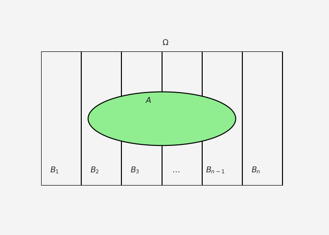
The key assumption in Naive Bayes is the conditional independence of features. Specifically, it assumes that the likelihood of each feature is independent of the others, given the class label:
\[ P(X_1, X_2, \dots, X_n | y) = P(X_1 | y) \cdot P(X_2 | y) \cdot \dots \cdot P(X_n | y) \]
While this assumption is often violated in real-world data, Naive Bayes can still perform well, especially when certain features dominate the prediction.
Requirements:
- Numerical Data: Naive Bayes can handle both numerical and categorical data, though different versions (Gaussian, Multinomial, Bernoulli) of the algorithm handle specific types of data more effectively
- Non-Collinear Features: Highly correlated features can distort predictions since the model assumes independence.
- Sufficient Data: Naive Bayes relies on probability estimates; thus, insufficient data might lead to unreliable predictions.
Types of Naive Bayes Classifiers
There are several variants of Naive Bayes, depending on the nature of the data:
- Gaussian Naive Bayes: Assumes features follow a Gaussian distribution (useful for continuous data).
- Multinomial Naive Bayes: Suitable for discrete data, often used in text classification (e.g., word counts).
- Bernoulli Naive Bayes: Works well for binary/boolean data, often used in scenarios where the features represent the presence/absence of a characteristic.
Mathematics behind the process
To understand the working of Naive Bayes, let’s start with the Bayes’s theorem
\[ P(y_k | X) = \frac{P(X|y_k) \cdot P(y_k)}{P(X)} \]
Where \(y_k\) is one of the possible classes. Due to the independence assumption, the likelihood term \(P(X|y_k)\) can be factorized as:
\[ P(X|y_k) = P(x_1|y_k) \cdot P(x_2|y_k) \cdot \dots \cdot P(x_n|y_k) \]
Where \(x_1, x_2, \dots, x_n\) are the individual features in the feature set \(X\). For each class \(y_k\), compute the posterior probability:
\[ P(y_k | X) \propto P(y_k) \cdot \prod_{i=1}^n P(x_i|y_k) \]
The denominator \(P(X)\) is constant for all classes, so we can ignore it during classification. Finally, the class \(y_k\) with the highest posterior probability is chosen as the predicted class:
\[\begin{align*} \hat{y} &= \arg\max_{y_k} P(y_k) \cdot \prod_{i=1}^n P(x_i|y_k)\\ \log{(\hat{y})}&= \log{ \left(\arg\max_{y_k} P(y_k) \cdot \prod_{i=1}^n P(x_i|y_k)\right)}\\ \implies \hat{y} & = \arg\max_{y_k} \left(\log P(y_k)+\sum_{i=1}^{n} P(x_i|y_k)\right) \end{align*}\]
Computing the probabilities
Prior Probabilities
\(P(y_k)\) is the prior probability, usually frequency of each class \(k\).
\[
P(y_k)=\frac{\text{number of instances in class }y_k}{\text{total number of instances}}
\]
Class Conditional Probabilities
\(P(x_i|y_k)\) is the class conditional probability. For the
Gaussian Naive Bayes: when the features are continuous and assumed that the features follow a Gaussian distribution, the
class conditionalprobability is given as \[ P(x_i|y_k) = \frac{1}{\sqrt{2\pi \sigma^2_k}}\exp{\left(-\frac{(x_i-\mu_i)^2}{2\sigma^2_k}\right)} \]Multinomial Naive Bayes: when the featrues (typically word frequencies) follow a multinomial distribution, the
class conditionaldistribution is given as
\[ P(x_i|y_k)=\frac{N_{x_i,y_k}+\alpha}{N_{y_k}+\alpha V} \]where,
- \(N_{x_i,y_k}\) is the count of the feature (e.g. word or term) \(x_i\) appearing in documents of class \(y_k\)
- \(N_{y_k}\) is the total count of all features (e.g. words) in all documents belonging to class \(y_k\)
- \(\alpha\) is a smoothing parameter (often called Laplace smoothing), used to avoid zero probabilities. If not using smoothing, set \(\alpha=0\)
- \(V\) is the size of the vocabulary (i.e., the number of unique words)
- \(N_{x_i,y_k}\) is the count of the feature (e.g. word or term) \(x_i\) appearing in documents of class \(y_k\)
Bernoulli Naive Bayes: when features are binary/boolean data, often used in scenarios where the features represent the presence/absence of a characteristic, the
class conditionaldistribution is given as
\[ P(x_i|y_k)=\begin{cases}\frac{N_{x_i,y_k}+\alpha}{N_{y_k}+2\alpha }\hspace{2mm}\text{ if } x_i=1\\ 1-\frac{N_{x_i,y_k}+\alpha}{N_{y_k}+2\alpha }\hspace{2mm}\text{ if } x_i=0\end{cases} \]
Python Implementation
Gaussian Naive Bayes
Code credit for the custom classifier goes to Assembly AI
Let’s apply this to the irish data set
import pandas as pd
from sklearn.datasets import load_iris


# Load Iris dataset
data = load_iris()
X = data.data  # Features
y = data.target  # Target variable (Classes)
df = pd.DataFrame(X, columns=data.feature_names)
df['target'] = pd.Categorical.from_codes(y, data.target_names)
df.head()| sepal length (cm) | sepal width (cm) | petal length (cm) | petal width (cm) | target | |
|---|---|---|---|---|---|
| 0 | 5.1 | 3.5 | 1.4 | 0.2 | setosa |
| 1 | 4.9 | 3.0 | 1.4 | 0.2 | setosa |
| 2 | 4.7 | 3.2 | 1.3 | 0.2 | setosa |
| 3 | 4.6 | 3.1 | 1.5 | 0.2 | setosa |
| 4 | 5.0 | 3.6 | 1.4 | 0.2 | setosa |
from sklearn.model_selection import train_test_split
from sklearn.naive_bayes import GaussianNB
from sklearn.metrics import accuracy_score, confusion_matrix, classification_report

# Split into training and testing sets
X_train, X_test, y_train, y_test = train_test_split(X, y, test_size=0.3, random_state=42)

gnb1 = GNaiveBayes()
gnb1.fit(X_train, y_train)
pred1 = gnb1.predict(X_test)
# Evaluate the model
acc1 = accuracy_score(y_test, pred1)

gnb2 = GaussianNB()
gnb2.fit(X_train, y_train)
pred2 = gnb2.predict(X_test)
acc2 = accuracy_score(y_test, pred2)

print('Accuracy from custom classifier = {:.2f}'.format(acc1*100))

# Confusion matrix and classification report
print(confusion_matrix(y_test, pred1))
print(classification_report(y_test, pred1))
print('\n')
print('Accuracy from sklearn classifier = {:.2f}'.format(acc2*100))
print(confusion_matrix(y_test, pred2))
print(classification_report(y_test, pred2))
Accuracy from custom classifier = 97.78
[[19 0 0]
[ 0 12 1]
[ 0 0 13]]
precision recall f1-score support
0 1.00 1.00 1.00 19
1 1.00 0.92 0.96 13
2 0.93 1.00 0.96 13
accuracy 0.98 45
macro avg 0.98 0.97 0.97 45
weighted avg 0.98 0.98 0.98 45
Accuracy from sklearn classifier = 97.78
[[19 0 0]
[ 0 12 1]
[ 0 0 13]]
precision recall f1-score support
0 1.00 1.00 1.00 19
1 1.00 0.92 0.96 13
2 0.93 1.00 0.96 13
accuracy 0.98 45
macro avg 0.98 0.97 0.97 45
weighted avg 0.98 0.98 0.98 45
Multinomial Naive Bayes
class MNaiveBayes:
    def __init__(self, alpha = 1):
        self.alpha = alpha

    def fit(self, X,y):
        """
        Fit the Multinomial Naive Bayes model to the training data.
        X: input data (n_samples, n_features)
        y: target labels (n_samples)
        """
        n_samples, n_features = X.shape
        self._classes = np.unique(y)
        n_classes = len(self._classes)

        # Initialize and count priors
        self._class_feature_count = np.zeros((n_classes, n_features),dtype=np.float64)
        self._class_count = np.zeros(n_classes, dtype=np.float64)
        self._prior = np.zeros(n_classes, dtype=np.float64)

        for idx,c in enumerate(self._classes):
            X_c = X[y==c]
            self._class_feature_count[idx,:] = X_c.sum(axis=0)
            self._class_count[idx] = X_c.shape[0]
            self._prior[idx] = X_c.shape[0]/float(n_samples)

        # Total count of all features accross all classes
        self._total_feature_count = self._class_feature_count.sum(axis=1)

    def predict(self, X):
        y_pred = [self._predict(x) for x in X]
        return np.array(y_pred)

    def _predict(self,x):
        posteriors = []
        for idx, c in enumerate(self._classes):
            prior = np.log(self._prior[idx])
            likelihood = np.sum(np.log(self._likelihood(idx,x)))
            posterior_prob = prior+ likelihood
            posteriors.append(posterior_prob)
        return self._classes[np.argmax(posteriors)]

    def _likelihood(self, class_idx, x):
        alpha = self.alpha
        V = len(self._class_feature_count[class_idx])
        class_feature_count = self._class_feature_count[class_idx]
        total_class_count = self._total_feature_count[class_idx]
        likelihood = (class_feature_count+alpha)/(total_class_count + alpha * V)

        return likelihood**x

X = np.array([[2, 1, 0],
              [1, 0, 1],
              [0, 3, 0],
              [2, 2, 1],
              [0, 0, 2]])

# Corresponding labels (2 classes: 0 and 1)
y = np.array([0, 1, 0, 0, 1])

# Create and train Multinomial Naive Bayes model
model = MNaiveBayes()
model.fit(X, y)

# Predict for new sample
X_test = np.array([[1, 1, 0], [0, 1, 1]])
predictions = model.predict(X_test)
print(predictions)
[0 0]Pros and Cons of Naive Bayes
Pros:
- Simplicity: Easy to implement and computationally efficient.
- Fast Training and Prediction: Naive Bayes is especially fast for both training and inference, even on large datasets.
- Performs Well with Small Data: Despite its simplicity, Naive Bayes works well even with relatively small datasets.
- Handles Irrelevant Features: Naive Bayes can often ignore irrelevant features in the data since the independence assumption dilutes their influence.
- Multi-Class Classification: Naturally suited for multi-class classification problems.
Cons:
- Strong Assumption of Independence: The assumption that features are independent is rarely true in real-world data, which can limit the model’s effectiveness.
- Poor Estimation of Probabilities: When dealing with very small datasets or unseen feature combinations, Naive Bayes can yield inaccurate probability estimates.
- Zero-Frequency Problem: If a feature value was not present in the training data, Naive Bayes will assign zero probability to the entire class, which can be addressed using Laplace smoothing.
Citation
@online{islam2024,
  author = {Islam, Rafiq},
  title = {Classification Using {Naive} {Bayes} Algorithm},
  date = {2024-10-10},
  url = {https://mrislambd.github.io/dsandml/naivebayes/},
  langid = {en}
}


