import numpy as np
import matplotlib.pyplot as plt
from sklearn.cluster import KMeans
from sklearn.datasets import make_blobs
from sklearn.metrics import silhouette_score

# For plotting purposes
import seaborn as sns
sns.set()Unsupervised Learning: K-Means Clustering
Introduction
Clustering is a fundamental technique in unsupervised learning where the goal is to group similar data points into clusters. One of the most popular algorithms for clustering is K-Means. K-Means is a centroid-based algorithm that partitions the dataset into \(k\) clusters. The algorithm iterates over data points, assigning each to one of \(k\) centroids (cluster centers), and then updates the centroids based on the current assignments. The objective is to minimize the sum of squared distances (also known as inertia) between each data point and its assigned centroid.
Mathematics Behind K-Means
The K-Means algorithm works through the following key steps:
Initialization: Randomly select \(k\) points from the dataset as initial centroids.
Assignment Step: For each data point, assign it to the closest centroid based on the Euclidean distance:
\[ \text{distance}(x_i, \mu_j) = \sqrt{\sum_{d=1}^{D} (x_i^d - \mu_j^d)^2} \]
where:
- \(x_i\) is the i-th data point.
- \(\mu_j\) is the j-th centroid.
- \(D\) is the number of features (dimensions).
Update Step: After all data points are assigned, recalculate the centroid of each cluster as the mean of all data points assigned to it:
\[ \mu_j = \frac{1}{n_j} \sum_{i=1}^{n_j} x_i \] where \(n_j\) is the number of points in cluster
j.Repeat: The assignment and update steps are repeated until the centroids no longer change or the maximum number of iterations is reached.
Objective Function (Inertia)
The objective of K-Means is to minimize the following cost function, also called inertia or within-cluster sum of squares:
\[ J = \sum_{j=1}^{k} \sum_{i=1}^{n_j} \|x_i - \mu_j\|^2 \]
This measures how compact the clusters are, i.e., how close the points within each cluster are to their centroid.
How to Choose the Best \(k\) Value?
One of the critical tasks in K-Means clustering is selecting the optimal number of clusters (\(k\)). Several methods can be used:
1. The Elbow Method
The most common way to determine the best \(k\) is the elbow method. It involves plotting the inertia (the sum of squared distances from each point to its assigned cluster centroid) for different values of \(k\). The point where the inertia starts to flatten out (forming an elbow) is considered a good choice for \(k\).
2. Silhouette Score
The silhouette score measures how similar each point is to its own cluster (cohesion) compared to other clusters (separation). It ranges from -1 to 1:
- \(1\) indicates that the point is well inside its cluster.
- \(0\) means the point is on the boundary between two clusters.
- Negative values indicate the point may have been assigned to the wrong cluster.
3. Gap Statistic
The gap statistic compares the total within-cluster variation for different values of \(k\) with the expected value under null reference distribution. The optimal number of clusters is where the gap statistic is the largest.
Python Implementation of K-Means
Synthetic Data
Let’s implement K-Means clustering using Python with visualizations and explore how to choose the best value of \(k\) using the elbow method.
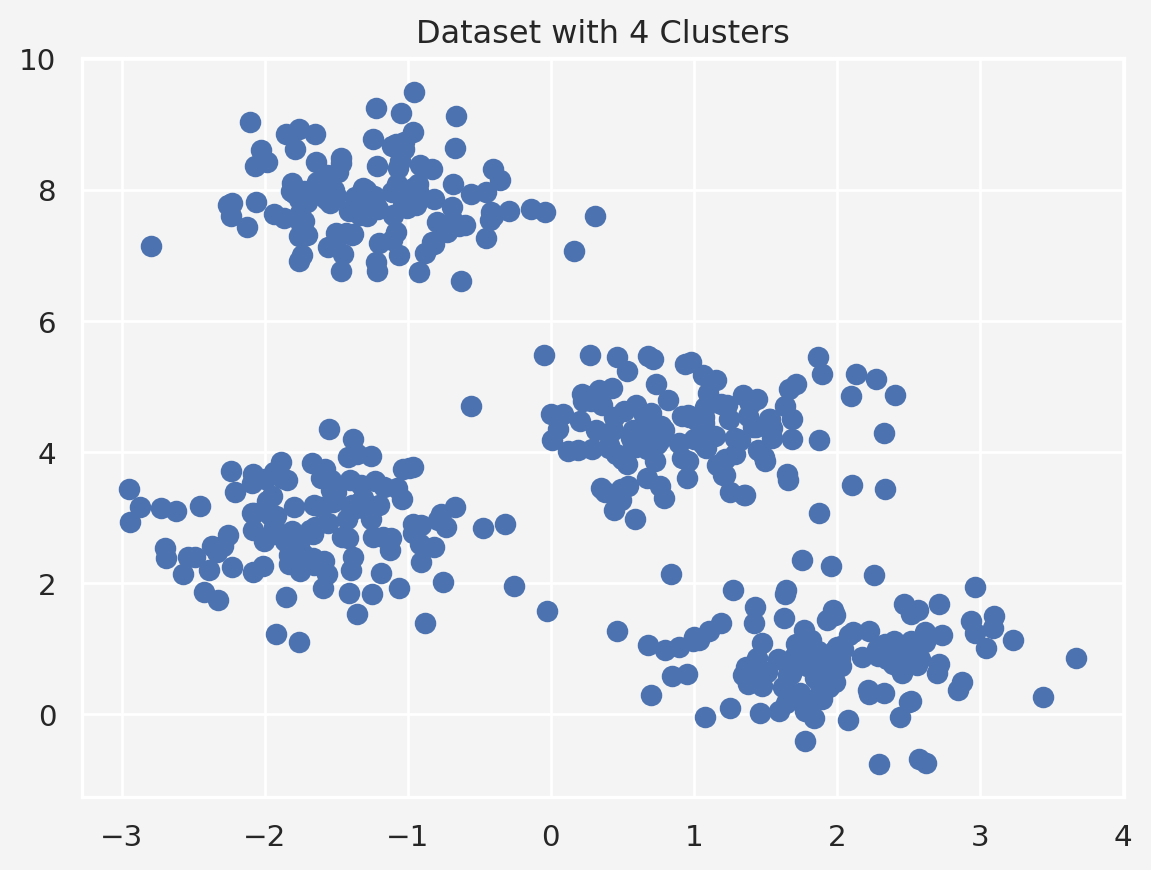
We’ll create a simple dataset with 4 distinct clusters for visualization.
# Create a dataset with 4 clusters
X, y = make_blobs(n_samples=500, centers=4, cluster_std=0.60, random_state=0)

# Visualize the dataset
plt.scatter(X[:, 0], X[:, 1], s=50)
plt.title('Dataset with 4 Clusters')
plt.gca().set_facecolor('#f4f4f4')
plt.gcf().patch.set_facecolor('#f4f4f4')
plt.show()
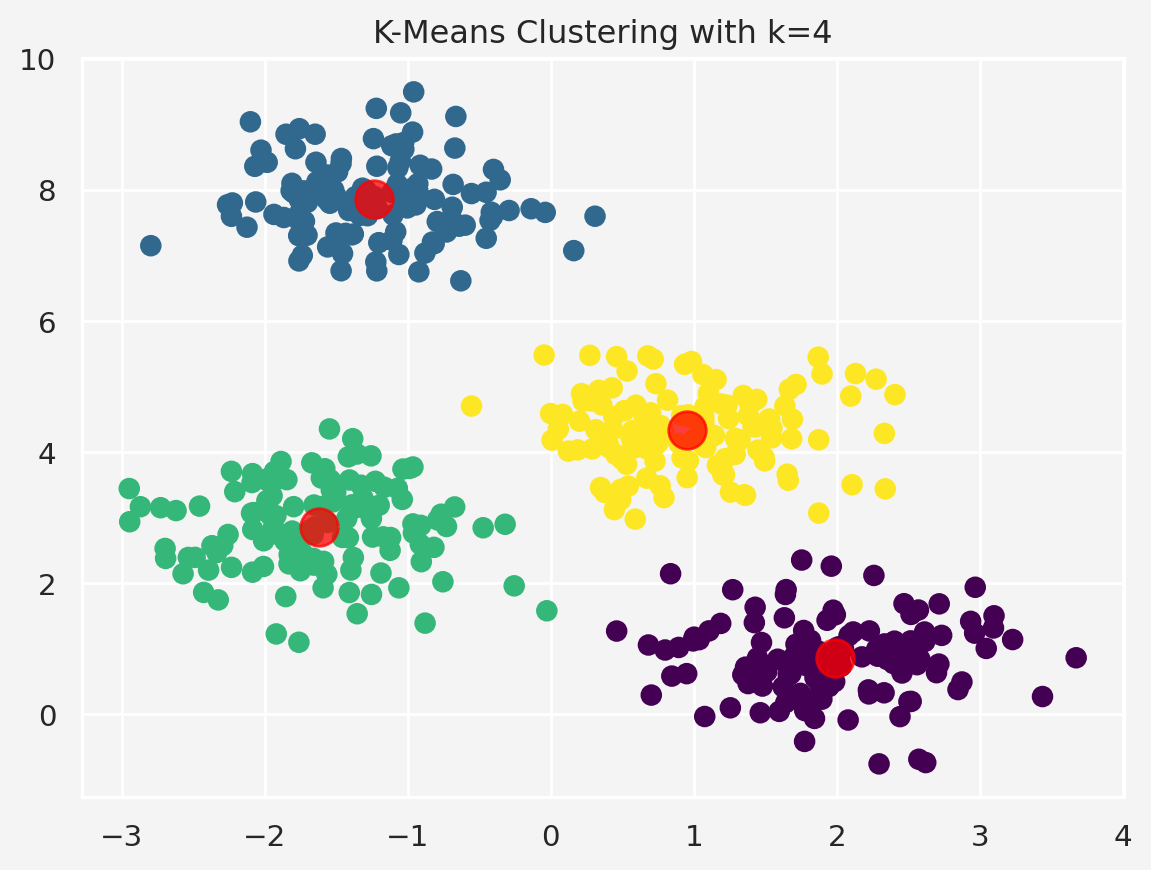
We can now apply K-Means clustering with different values of \(k\) and observe how the clusters are formed.
# Fit KMeans with k=4 (since we know we generated 4 clusters)
kmeans = KMeans(n_clusters=4)
kmeans.fit(X)

# Predict clusters
y_kmeans = kmeans.predict(X)

# Plot the clustered data
plt.scatter(X[:, 0], X[:, 1], c=y_kmeans, s=50, cmap='viridis')

# Plot the centroids
centers = kmeans.cluster_centers_
plt.scatter(centers[:, 0], centers[:, 1], c='red', s=200, alpha=0.75)
plt.title('K-Means Clustering with k=4')
plt.savefig('kmeans.png')
plt.gca().set_facecolor('#f4f4f4')
plt.gcf().patch.set_facecolor('#f4f4f4')
plt.show()
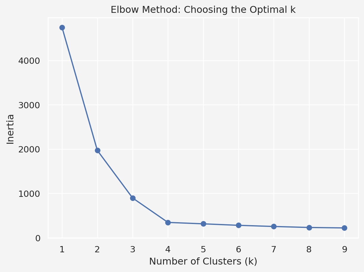
To determine the optimal number of clusters, we’ll plot the inertia for different values of \(k\) using the elbow method.
# Test multiple k values
inertia = []
k_values = range(1, 10)

for k in k_values:
    kmeans = KMeans(n_clusters=k)
    kmeans.fit(X)
    inertia.append(kmeans.inertia_)

# Plot the inertia vs. k values
plt.plot(k_values, inertia, marker='o')
plt.title('Elbow Method: Choosing the Optimal k')
plt.xlabel('Number of Clusters (k)')
plt.ylabel('Inertia')
plt.gca().set_facecolor('#f4f4f4')
plt.gcf().patch.set_facecolor('#f4f4f4')
plt.show()
We see that the curve starts to flatten at \(k=4\), suggesting this is a good choice for the number of clusters. Let’s also compute the silhouette score for different values of \(k\) to confirm our choice.
sil_scores = []
for k in range(2, 10):
    kmeans = KMeans(n_clusters=k)
    kmeans.fit(X)
    labels = kmeans.predict(X)
    sil_scores.append(silhouette_score(X, labels))

# Plot Silhouette Score vs. k
plt.plot(range(2, 10), sil_scores, marker='o')
plt.title('Silhouette Score for Different k Values')
plt.xlabel('Number of Clusters (k)')
plt.ylabel('Silhouette Score')
plt.gca().set_facecolor('#f4f4f4')
plt.gcf().patch.set_facecolor('#f4f4f4')
plt.show()
Real Data
Description:This dataset contains information about customers of a shopping mall, including their annual income, spending score, gender, and age.
Goal: Our goal is to segment customers into different groups based on their spending behavior and income.
Columns:
- CustomerID: Unique identifier for each customer.
- Gender: The gender of the customer (Male or Female).
- Age: Age of the customer.
- Annual Income: Annual income of the customer in thousands of dollars.
- Spending Score: A score assigned by the mall based on customer behavior and spending patterns.
Data Source: You can find the Mall Customer Segmentation data on Kaggle.
import pandas as pd
mall = pd.read_csv('Mall_Customers.csv')
mall.head()| CustomerID | Gender | Age | Annual Income (k$) | Spending Score (1-100) | |
|---|---|---|---|---|---|
| 0 | 1 | Male | 19 | 15 | 39 |
| 1 | 2 | Male | 21 | 15 | 81 |
| 2 | 3 | Female | 20 | 16 | 6 |
| 3 | 4 | Female | 23 | 16 | 77 |
| 4 | 5 | Female | 31 | 17 | 40 |
# Data Information
print(mall.info())
print('\n')
# Check for Missing Data
print(mall.isnull().sum())
print('\n')
# Data Description
mall.rename(columns={'CustomerID':'ID','Annual Income (k$)':'Income','Spending Score (1-100)':'SpendingScore'},inplace=True)
cmall = mall.drop('ID',axis=1)
print(cmall.describe().loc[['mean','std','min','max']].T)
<class 'pandas.core.frame.DataFrame'>
RangeIndex: 200 entries, 0 to 199
Data columns (total 5 columns):
# Column Non-Null Count Dtype
--- ------ -------------- -----
0 CustomerID 200 non-null int64
1 Gender 200 non-null object
2 Age 200 non-null int64
3 Annual Income (k$) 200 non-null int64
4 Spending Score (1-100) 200 non-null int64
dtypes: int64(4), object(1)
memory usage: 7.9+ KB
None
CustomerID 0
Gender 0
Age 0
Annual Income (k$) 0
Spending Score (1-100) 0
dtype: int64
mean std min max
Age 38.85 13.969007 18.0 70.0
Income 60.56 26.264721 15.0 137.0
SpendingScore 50.20 25.823522 1.0 99.0Pre-Process: Since our data contains categorical variable Gender, we need to encode this column and scale the numerical features like Age, Annual Income, and Spending Score.
from sklearn.preprocessing import StandardScaler
X = mall[['Age','Income','SpendingScore']]
scaler = StandardScaler()
X_scaled = scaler.fit_transform(X)
print(X_scaled[:5])
[[-1.42456879 -1.73899919 -0.43480148]
[-1.28103541 -1.73899919 1.19570407]
[-1.3528021 -1.70082976 -1.71591298]
[-1.13750203 -1.70082976 1.04041783]
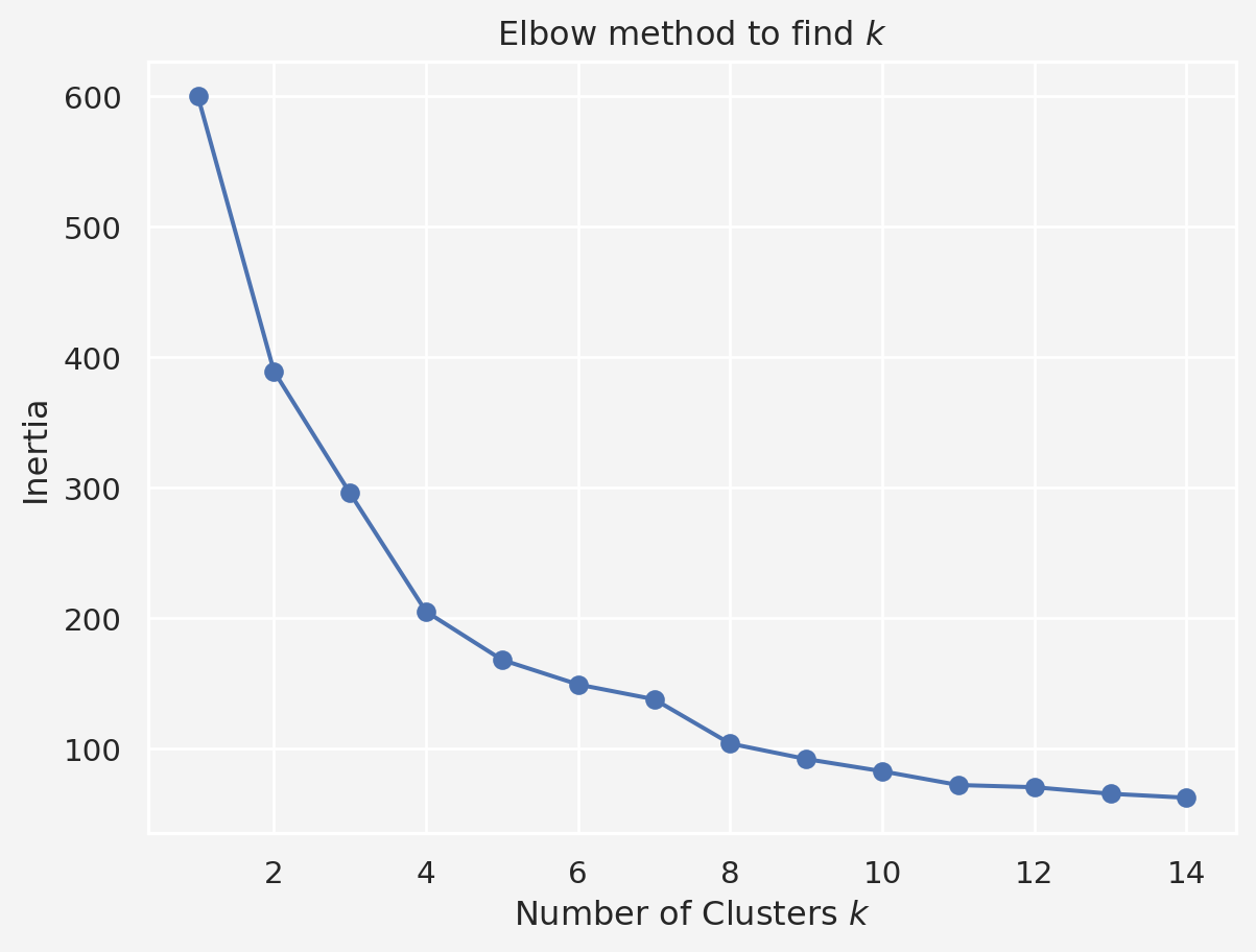
[-0.56336851 -1.66266033 -0.39597992]]Next we use the Elbow method to find the best \(k\), the number of clusters
k_values = range(1,15)
inertia = []
for k in k_values:
    kmeans = KMeans(n_clusters=k, random_state=123)
    kmeans.fit(X_scaled)
    inertia.append(kmeans.inertia_)
plt.plot(k_values,inertia, marker='o')
plt.title('Elbow method to find $k$')
plt.xlabel('Number of Clusters $k$')
plt.ylabel('Inertia')
plt.gca().set_facecolor('#f4f4f4')
plt.gcf().patch.set_facecolor('#f4f4f4')
plt.show()
The elbow point in the plot (where the decrease in inertia starts to slow) helps determine the optimal number of clusters. Let’s say we find that \(k=5\) looks like a reasonable choice from the plot.
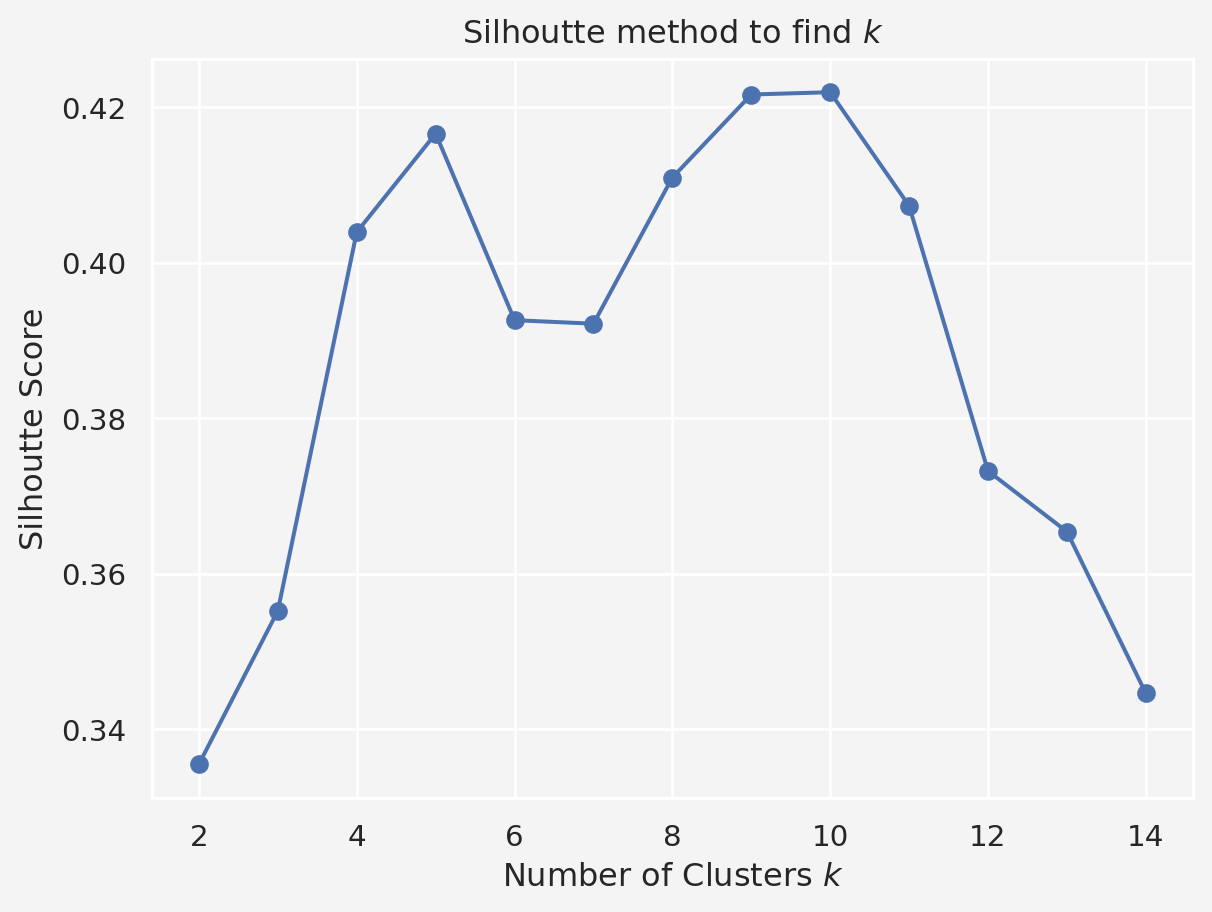
To further validate the choice of \(k\), let’s compute the silhouette score for different cluster numbers. A higher silhouette score indicates better-defined clusters
sil_scores = []
for k in range(2,15):
    kmeans = KMeans(n_clusters=k, random_state=123)
    labels = kmeans.fit_predict(X_scaled)
    sil_scores.append(silhouette_score(X_scaled,labels))
plt.plot(range(2,15),sil_scores, marker='o')
plt.title('Silhoutte method to find $k$')
plt.xlabel('Number of Clusters $k$')
plt.ylabel('Silhoutte Score')
plt.gca().set_facecolor('#f4f4f4')
plt.gcf().patch.set_facecolor('#f4f4f4')
plt.show()
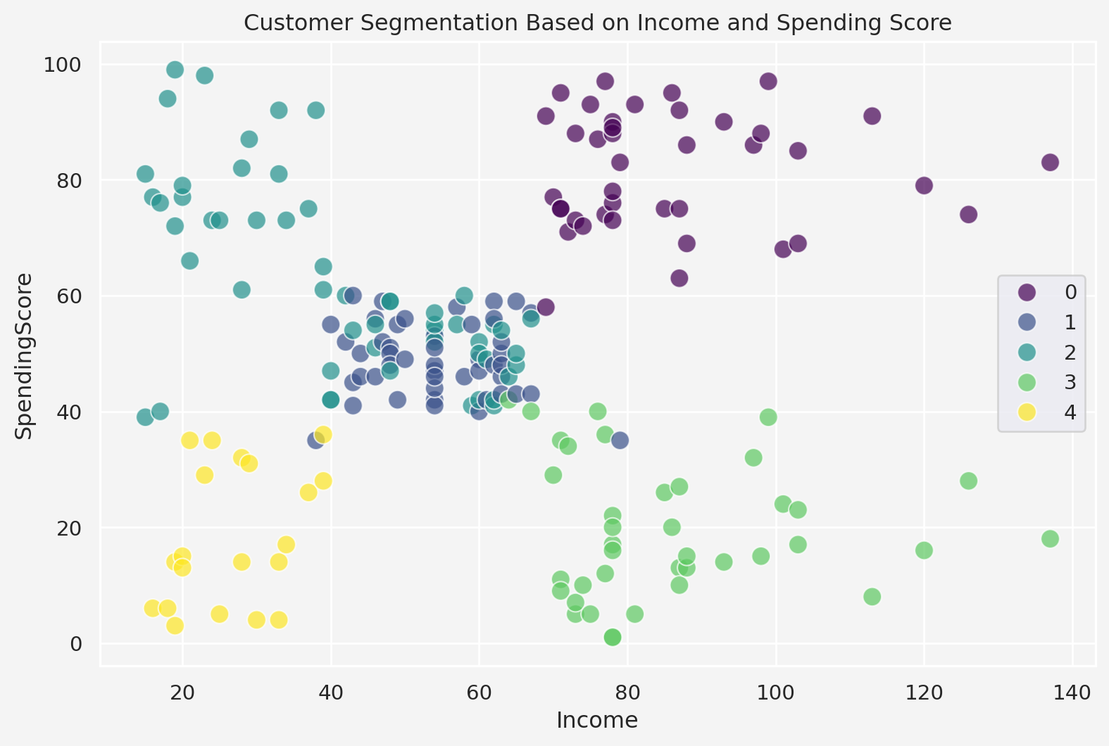
Next, we apply \(k=5\) clusters
plt.figure(figsize=(9.5,6))
kmeans = KMeans(n_clusters=5, random_state=123)
mall['Cluster'] = kmeans.fit_predict(X_scaled)
print(mall.head())
sns.scatterplot(
    x='Income', y='SpendingScore', hue='Cluster',
    data=mall, palette='viridis', s=100, alpha=0.7
    )
plt.title('Customer Segmentation Based on Income and Spending Score')
plt.legend()
plt.gca().set_facecolor('#f4f4f4')
plt.gcf().patch.set_facecolor('#f4f4f4')
plt.show()
ID Gender Age Income SpendingScore Cluster
0 1 Male 19 15 39 2
1 2 Male 21 15 81 2
2 3 Female 20 16 6 4
3 4 Female 23 16 77 2
4 5 Female 31 17 40 2Analyze the segments
cluster_summary = mall.drop(columns=['Gender','ID']).groupby('Cluster').mean()
print(cluster_summary)
Age Income SpendingScore
Cluster
0 32.875000 86.100000 81.525000
1 55.638298 54.382979 48.851064
2 25.185185 41.092593 62.240741
3 39.871795 86.102564 19.358974
4 46.250000 26.750000 18.350000Now say we have two new customers
new_customer = {'ID':[201,202],'Gender':['Male','Female'],'Age': [30,50],'Income':[40,70],'SpendingScore':[70,20]}
new_customer = pd.DataFrame(new_customer)
print(new_customer)
ID Gender Age Income SpendingScore
0 201 Male 30 40 70
1 202 Female 50 70 20We would like to know in which cluster they belong.
X_new = new_customer[['Age', 'Income','SpendingScore']]
X_new_sc = scaler.transform(X_new)
cluster_labels = kmeans.predict(X_new_sc)
print(cluster_labels)
[2 3]K-Means is a powerful and widely used clustering algorithm, but it has limitations, such as assuming spherical clusters of equal sizes.
Limitations of K-Means Clustering
While K-Means is a widely used clustering algorithm due to its simplicity and scalability, it has several notable limitations:
1. Assumption of Spherical Clusters
K-Means assumes that clusters are spherical and have roughly the same size. This assumption may not hold true in real-world datasets, where clusters may have different shapes and densities. For example, if clusters are elongated or irregularly shaped, K-Means may not perform well.
- Solution: Use algorithms like DBSCAN (Density-Based Spatial Clustering of Applications with Noise) or Spectral Clustering, which do not assume any specific shape for the clusters.
2. Sensitivity to Initialization
K-Means is sensitive to the initial selection of centroids. Different initializations can lead to different final clusters, and in some cases, the algorithm may converge to suboptimal solutions. To address this, the algorithm is often run multiple times with different initializations (e.g., using the k-means++ initialization method).
- Solution: Use the
k-means++initialization, which ensures that centroids are chosen in a way that increases the likelihood of converging to an optimal solution.
3. Needs to Specify k in Advance
One of the main limitations is that K-Means requires the number of clusters (k) to be specified in advance. This can be a challenge when the number of clusters is unknown, and choosing the wrong k can lead to poor clustering results.
- Solution: Use the Elbow Method, Silhouette Score, or the Gap Statistic to estimate the best value for
k.
4. Outliers and Noise Sensitivity
K-Means is highly sensitive to outliers, as they can significantly affect the position of centroids. An outlier will either form its own cluster or distort the positions of nearby centroids, leading to incorrect clustering.
- Solution: Preprocess your data by removing outliers or use clustering methods like DBSCAN, which can handle outliers more effectively by considering them as noise.
5. Equal Cluster Size Assumption
The algorithm tends to assign roughly equal-sized clusters because it minimizes variance. This can be a problem if clusters in your data have highly varying sizes. Small clusters might be absorbed into larger ones.
- Solution: Use Hierarchical Clustering, which can naturally handle different cluster sizes.
6. Non-Convex Shapes
K-Means struggles with data where clusters have non-convex shapes, such as two overlapping rings or crescent shapes. It partitions the space into Voronoi cells, which are convex, leading to poor clustering results in non-convex structures.
- Solution: Algorithms like Spectral Clustering or Gaussian Mixture Models (GMM) can better handle non-convex clusters.
References
- K-Means Algorithm:
- MacQueen, J. B. (1967). “Some Methods for Classification and Analysis of Multivariate Observations”. Proceedings of the Fifth Berkeley Symposium on Mathematical Statistics and Probability, Volume 1: Statistics.
- Hartigan, J. A., & Wong, M. A. (1979). “Algorithm AS 136: A K-means clustering algorithm”. Journal of the Royal Statistical Society. Series C (Applied Statistics), 28(1), 100-108.
- Choosing
k(Elbow Method & Silhouette Score):- Rousseeuw, P. J. (1987). “Silhouettes: A graphical aid to the interpretation and validation of cluster analysis”. Journal of Computational and Applied Mathematics, 20, 53-65.
- Inertia and the Elbow Method:
- Tibshirani, R., Walther, G., & Hastie, T. (2001). “Estimating the number of clusters in a dataset via the gap statistic”. Journal of the Royal Statistical Society: Series B (Statistical Methodology), 63(2), 411-423.
Share on
You may also like
Citation
@online{islam2024,
  author = {Islam, Rafiq},
  title = {Unsupervised {Learning:} {K-Means} {Clustering}},
  date = {2024-09-28},
  url = {https://mrislambd.github.io/dsandml/kmeans/},
  langid = {en}
}
