Exploratory Data Analysis (EDA) and Data Visualization

In this Exploratory Data Analysis and Visualization notebook, we want to explore the 911 call data from Kaggle.com

The Dataset

import pandas as pd
import numpy as np
import seaborn as sns
import matplotlib.pyplot as plt
df = pd.read_csv('911.csv')

Discriptive Statistics

We first check the data information to see the number of observations, datatype, memory usages etc.

df.info()

<class 'pandas.core.frame.DataFrame'>
RangeIndex: 105957 entries, 0 to 105956
Data columns (total 9 columns):
 #   Column     Non-Null Count   Dtype  
---  ------     --------------   -----  
 0   lat        105957 non-null  float64
 1   lng        105957 non-null  float64
 2   desc       105957 non-null  object 
 3   zip        92735 non-null   float64
 4   title      105957 non-null  object 
 5   timeStamp  105957 non-null  object 
 6   twp        105924 non-null  object 
 7   addr       105957 non-null  object 
 8   e          105957 non-null  int64  
dtypes: float64(3), int64(1), object(5)
memory usage: 7.3+ MB

A first look of the data

df.head()

	lat	lng	desc	zip	title	timeStamp	twp	addr	e
0	40.297876	-75.581294	REINDEER CT & DEAD END; NEW HANOVER; Station ...	19525.0	EMS: BACK PAINS/INJURY	12/10/15 17:10	NEW HANOVER	REINDEER CT & DEAD END	1
1	40.258061	-75.264680	BRIAR PATH & WHITEMARSH LN; HATFIELD TOWNSHIP...	19446.0	EMS: DIABETIC EMERGENCY	12/10/15 17:29	HATFIELD TOWNSHIP	BRIAR PATH & WHITEMARSH LN	1
2	40.121182	-75.351975	HAWS AVE; NORRISTOWN; 2015-12-10 @ 14:39:21-St...	19401.0	Fire: GAS-ODOR/LEAK	12/10/15 14:39	NORRISTOWN	HAWS AVE	1
3	40.116153	-75.343513	AIRY ST & SWEDE ST; NORRISTOWN; Station 308A;...	19401.0	EMS: CARDIAC EMERGENCY	12/10/15 16:47	NORRISTOWN	AIRY ST & SWEDE ST	1
4	40.251492	-75.603350	CHERRYWOOD CT & DEAD END; LOWER POTTSGROVE; S...	NaN	EMS: DIZZINESS	12/10/15 16:56	LOWER POTTSGROVE	CHERRYWOOD CT & DEAD END	1

Some data related questions. For example,

• What are the top 10 zipcodes for 911 calls?

  df.zip.value_counts().head(10)

  zip
  19401.0    7445
  19464.0    7122
  19403.0    5189
  19446.0    5060
  19406.0    3404
  19002.0    3238
  19468.0    3202
  19454.0    2984
  19090.0    2832
  19046.0    2779
  Name: count, dtype: int64

• What are the top 10 twonships for the 911 calls?

  df.twp.value_counts().head(10)

  twp
  LOWER MERION        9069
  ABINGTON            6403
  NORRISTOWN          6265
  UPPER MERION        5551
  CHELTENHAM          4882
  POTTSTOWN           4448
  UPPER MORELAND      3658
  LOWER PROVIDENCE    3435
  PLYMOUTH            3371
  HORSHAM             3142
  Name: count, dtype: int64

Feature Engineering

Sometimes creating new features from the existing features helps understand the data better. For example, for this dataset, we can create a new column called Reason for emergency 911 call.

df['reason'] = df.title.apply(lambda title: title.split(':')[0])
df.head(3)

	lat	lng	desc	zip	title	timeStamp	twp	addr	e	reason
0	40.297876	-75.581294	REINDEER CT & DEAD END; NEW HANOVER; Station ...	19525.0	EMS: BACK PAINS/INJURY	12/10/15 17:10	NEW HANOVER	REINDEER CT & DEAD END	1	EMS
1	40.258061	-75.264680	BRIAR PATH & WHITEMARSH LN; HATFIELD TOWNSHIP...	19446.0	EMS: DIABETIC EMERGENCY	12/10/15 17:29	HATFIELD TOWNSHIP	BRIAR PATH & WHITEMARSH LN	1	EMS
2	40.121182	-75.351975	HAWS AVE; NORRISTOWN; 2015-12-10 @ 14:39:21-St...	19401.0	Fire: GAS-ODOR/LEAK	12/10/15 14:39	NORRISTOWN	HAWS AVE	1	Fire

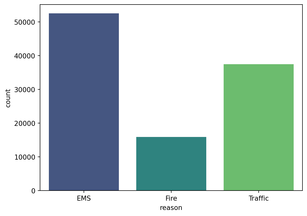
what are top reasons for the emergency calls?

df.reason.value_counts()

reason
EMS        52515
Traffic    37505
Fire       15937
Name: count, dtype: int64

visualization of the reason column

sns.countplot(x=df.reason, hue=df.reason, palette='viridis')

The timeStamp column contains time information year-month-day hour:minute:second format but in string value/object. So we can convert this column to obtain new features.

df['timeStamp'] = pd.to_datetime(df.timeStamp)
time = df.timeStamp.iloc[0]

/tmp/ipykernel_15019/1994586768.py:1: UserWarning:

Could not infer format, so each element will be parsed individually, falling back to `dateutil`. To ensure parsing is consistent and as-expected, please specify a format.

Let’s create new features called hour, month, and day of the calls.

df['hour'] = df.timeStamp.apply(lambda time: time.hour)
df['month'] = df.timeStamp.apply(lambda time: time.month)
df['day'] = df.timeStamp.apply(lambda time: time.dayofweek)
days = {
    0:'Monday', 1:'Tuesday', 2:'Wednesday', 
    3:'Thursday', 4:'Friday', 5:'Saturday',
    6:'Sunday'
    }
df.day = df.day.map(days)
df = df[
    ['lat','lng','zip','twp','e','reason',
    'month','day','hour','title','timeStamp',
    'desc','addr']
    ]
df.head(3)

	lat	lng	zip	twp	e	reason	month	day	hour	title	timeStamp	desc	addr
0	40.297876	-75.581294	19525.0	NEW HANOVER	1	EMS	12	Thursday	17	EMS: BACK PAINS/INJURY	2015-12-10 17:10:00	REINDEER CT & DEAD END; NEW HANOVER; Station ...	REINDEER CT & DEAD END
1	40.258061	-75.264680	19446.0	HATFIELD TOWNSHIP	1	EMS	12	Thursday	17	EMS: DIABETIC EMERGENCY	2015-12-10 17:29:00	BRIAR PATH & WHITEMARSH LN; HATFIELD TOWNSHIP...	BRIAR PATH & WHITEMARSH LN
2	40.121182	-75.351975	19401.0	NORRISTOWN	1	Fire	12	Thursday	14	Fire: GAS-ODOR/LEAK	2015-12-10 14:39:00	HAWS AVE; NORRISTOWN; 2015-12-10 @ 14:39:21-St...	HAWS AVE

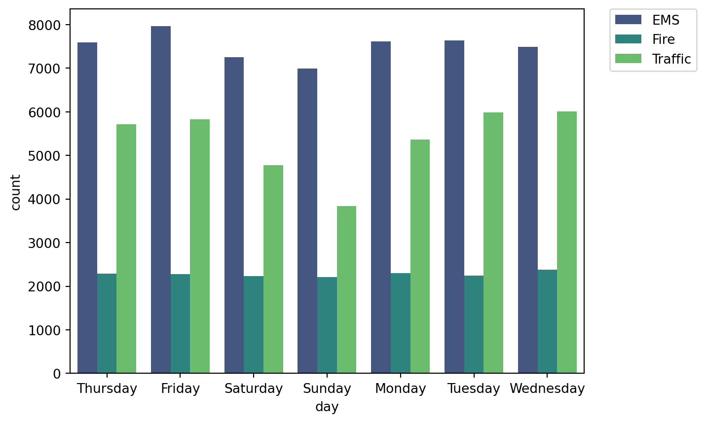
Now that we have almost a clean dataset, we can analyze the reason column based on the days of the week or months of a year.

sns.countplot(x='day', data= df, hue='reason', palette='viridis')
plt.legend(bbox_to_anchor=(1.05,1), loc=2, borderaxespad=0.0)

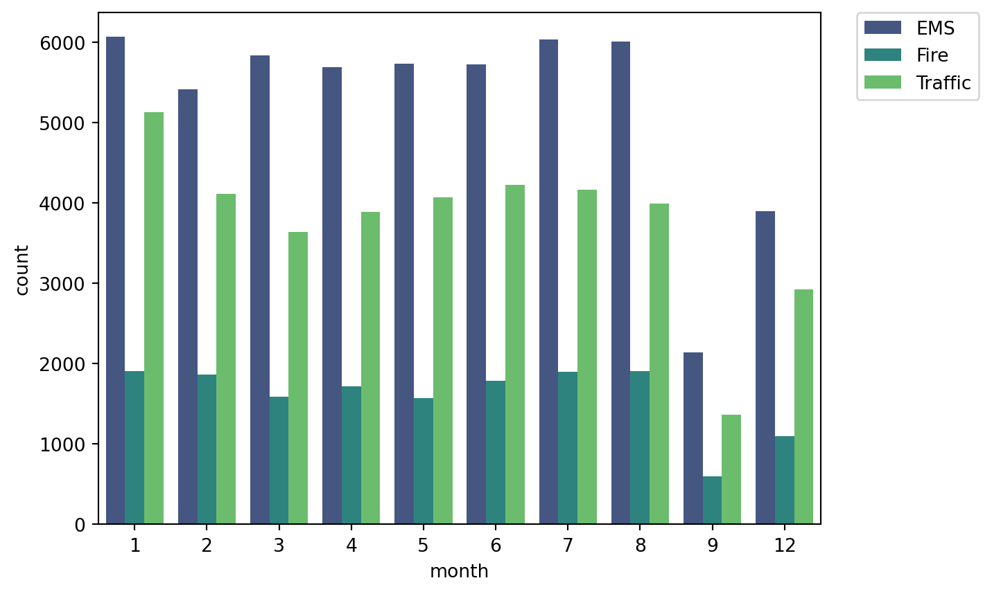
For the month column

sns.countplot(x='month', data= df, hue='reason', palette='viridis')
plt.legend(bbox_to_anchor=(1.05,1), loc=2, borderaxespad=0.0)

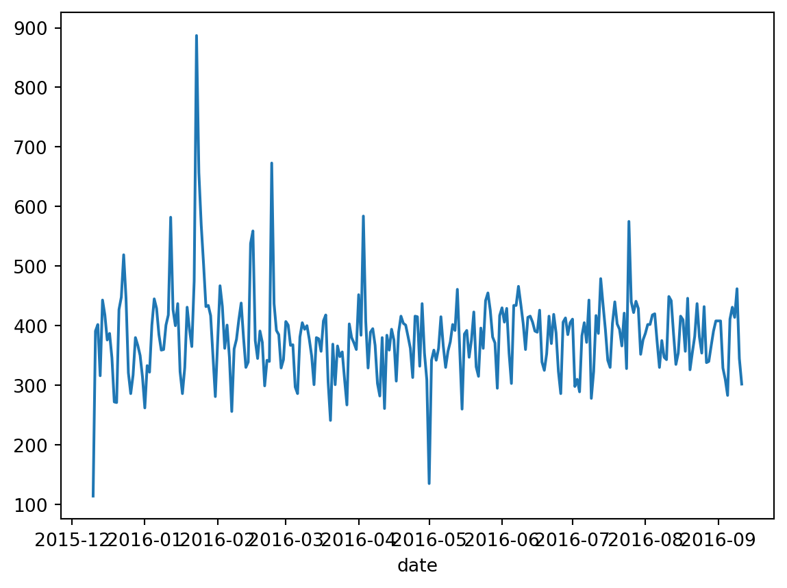
To create a time series data

df['date'] = df['timeStamp'].apply(lambda time: time.date())
df.groupby('date').count()['twp'].plot()

Now to see for each reason

start_date = pd.to_datetime('2019-01-01')


df['date'] = pd.to_datetime(df['date'])


fig = plt.figure(figsize=(7.9,6))

ax1 = fig.add_subplot(311)
df[(df['reason'] == 'Traffic') & (df['date'] >= start_date)].groupby('date').count()['twp'].plot(ax=ax1)

ax2 = fig.add_subplot(312)
df[(df['reason'] == 'Fire') & (df['date'] >= start_date)].groupby('date').count()['twp'].plot(ax=ax2)

ax3 = fig.add_subplot(313)
df[(df['reason'] == 'EMS') & (df['date'] >= start_date)].groupby('date').count()['twp'].plot(ax=ax3)

plt.tight_layout()

plt.show()

---

Share on

You may also like