In the world of data analysis and machine learning, statistics plays a vital role in making sense of the data. Whether you’re estimating parameters, testing hypotheses, or understanding relationships between variables, statistical concepts guide how we interpret data. In this post, I want to summarise and collect some fundamental statistical ideas that are quite common and asked in many data science, machine learning, and quant interviews
Basic Statistical Terminologies
The mean
The mean is one of the most basic statistical concepts and represents the average value of a dataset. It’s calculated by summing all the values in a dataset and then dividing by the number of observations.
Mathematically, for a set of discrete observations , the mean or Expected Value is defined as:
For a continuous random variable , the mean
where, is the probability mass function (pmf) and is the probability density function (pdf) of the random variable , depending on whether it is discrete or contineous type. The mean helps describe the central tendency of data, but it can be sensitive to outliers.
Variance
Variance measures the spread or dispersion of a dataset relative to its mean. It tells us how far the individual data points are from the mean. A small variance indicates that data points are clustered closely around the mean, while a large variance means they are spread out.
The formula for variance is:
However, the population and sample variance formula are slightly different. For discrete observations, the sample variance is given as
Instead of dividing by we devide by to have the sample variance unbiased and bigger than the population variance so that it contains the true population variance.
Examples
Normal Distribution with mean and variance has the pdf
Standard Normal Distribution with mean and variance has the pdf
Now if then what is the distribution of ?
Covariance
Covariance measures how two variables move together. If the covariance is positive, the two variables tend to increase or decrease together. If negative, one variable tends to increase when the other decreases.
The formula for covariance between two variables and is:
However, covariance doesn’t indicate the strength of the relationship, which brings us to correlation.
Correlation
Correlation is a standardized measure of the relationship between two variables. It ranges from to , where indicates a perfect positive relationship, a perfect negative relationship, and no relationship.
The most common correlation metric is Pearson correlation, defined as:
Unlike covariance, correlation gives a clearer picture of the strength and direction of a linear relationship between variables.
P-Values and Hypothesis Testing
P-values and hypothesis testing form the backbone of inferential statistics. Hypothesis testing is used to determine if a given assumption (the null hypothesis) about a population parameter is true or not.
The null hypothesis typically suggests no effect or no difference.
The alternative hypothesis is the claim you want to test.
The p-value is the probability of observing a result as extreme as, or more extreme than, the one obtained, assuming the null hypothesis is true. A small p-value (usually less than 0.05) indicates that the null hypothesis is unlikely, and we may reject it in favor of the alternative hypothesis.
Maximum Likelihood Estimation (MLE)
Maximum Likelihood Estimation (MLE) is a method for estimating the parameters of a statistical model. The idea behind MLE is to find the parameter values that maximize the likelihood function, which represents the probability of observing the given data under a particular model.
Given a parameter and observed data , the likelihood function is:
MLE finds the parameter that maximizes this likelihood:
MLE is widely used in statistical modeling, from simple linear regression to complex machine learning algorithms.
Maximum A Posteriori (MAP)
While MLE focuses on maximizing the likelihood, Maximum A Posteriori (MAP) estimation incorporates prior information about the parameters. MAP is rooted in Bayesian statistics, where the goal is to find the parameter that maximizes the posterior distribution.
The posterior is given by Bayes’ Theorem:
MAP finds the parameter that maximizes the posterior probability:
Unlike MLE, MAP estimation incorporates the prior distribution , making it more robust when prior knowledge is available
---title: "Some Key Statistical Concepts for Interview Prep"date: "05/09/2024"author: Rafiq Islamcategories: [Data Science, Machine Learning, Artificial Intelligence, Statistics]citation: truesearch: trueimage: stat.jpeglightbox: truelisting: contents: "/../../posts" max-items: 3 type: grid categories: false date-format: full fields: [image, date, title, author, reading-time]format: html: default ipynb: default docx: toc: true adsense: enable-ads: false epub: toc: true adsense: enable-ads: false pdf: toc: true pdf-engine: xelatex adsense: enable-ads: false number-sections: false colorlinks: truetoc-depth: 4---<p style="text-align:justify"> In the world of data analysis and machine learning, statistics plays a vital role in making sense of the data. Whether you're estimating parameters, testing hypotheses, or understanding relationships between variables, statistical concepts guide how we interpret data. In this post, I want to summarise and collect some fundamental statistical ideas that are quite common and asked in many data science, machine learning, and quant interviews</p>## Basic Statistical Terminologies ### The mean The **mean** is one of the most basic statistical concepts and represents the average value of a dataset. It’s calculated by summing all the values in a dataset and then dividing by the number of observations.Mathematically, for a set of discrete observations $x_1, x_2, ..., x_n$, the mean $\mu$ or *Expected Value* is defined as:\begin{align*}\mu &= \frac{1}{n} \sum_{i=1}^{n} x_i\\\implies \mathbb{E}[X] &= \sum_{i=1}^{n} x_i\mathbb{P}(X=x_i)\end{align*} For a continuous random variable $X$, the mean $$\mu = \mathbb{E}[X]=\int_{-\infty}^{\infty}xf_X(x)dx$$ <p style="text-align: justify"> where, $\mathbb{P}(X=x)$ is the *probability mass function (pmf)* and $f_X(x)$ is the *probability density function (pdf)* of the random variable $X$, depending on whether it is discrete or contineous type. The mean helps describe the central tendency of data, but it can be sensitive to outliers.</p>### Variance <p style="text-align: justify"> **Variance** measures the spread or dispersion of a dataset relative to its mean. It tells us how far the individual data points are from the mean. A small variance indicates that data points are clustered closely around the mean, while a large variance means they are spread out.</p>The formula for variance $\sigma^2$ is:\begin{align*} \sigma^2=Var(X)&=\frac{1}{n} \sum_{i=1}^{n} (x_i - \mu)^2\\ &=\mathbb{E}\left[(X-\mathbb{E}[X])^2\right]\\ &=\mathbb{E}\left[(X^2-2X\mathbb{E}[X]+(\mathbb{E}[X])^2)\right]\\ &=\mathbb{E}[X^2]-2\mathbb{E}[X]\mathbb{E}[X]+(\mathbb{E}[X])^2\\ &=\mathbb{E}[X^2]-(\mathbb{E}[X])^2\\\end{align*}However, the population and sample variance formula are slightly different. For discrete observations, the sample variance is given as $$ s= \frac{1}{n-1} \sum_{i=1}^{n} (x_i - \mu)^2$$Instead of dividing by $n$ we devide by $n-1$ to have the sample variance unbiased and bigger than the population variance so that it contains the true population variance. **Examples** 1. Normal Distribution with mean $\mu$ and variance $\sigma^2$ has the pdf $f_{X}(x)=\frac{1}{\sqrt{2\pi \sigma^2}}\exp{\left[-\frac{(x-\mu)^2}{2\sigma^2}\right]}$ 2. Standard Normal Distribution with mean $0$ and variance $1$ has the pdf $f_{X}(x)=\frac{1}{\sqrt{2\pi \sigma^2}}\exp{\left[-\frac{x^2}{2}\right]}$ 3. Now if $\log X\sim \mathbfcal{N}(0,1)$ then what is the distribution of $X$?### Covariance<p style="text-align: justify"> **Covariance** measures how two variables move together. If the covariance is positive, the two variables tend to increase or decrease together. If negative, one variable tends to increase when the other decreases.</p>The formula for covariance between two variables $X$ and $Y$ is:$$\text{Cov}(X, Y) = \frac{1}{n} \sum_{i=1}^{n} (X_i - \mu_X)(Y_i - \mu_Y)$$However, covariance doesn’t indicate the strength of the relationship, which brings us to **correlation**.### Correlation <p style="text-align: justify"> **Correlation** is a standardized measure of the relationship between two variables. It ranges from $-1$ to $1$, where $1$ indicates a perfect positive relationship, $-1$ a perfect negative relationship, and $0$ no relationship.</p>The most common correlation metric is **Pearson correlation**, defined as:$$\rho(X, Y) = \frac{\text{Cov}(X, Y)}{\sigma_X \sigma_Y}$$Unlike covariance, correlation gives a clearer picture of the strength and direction of a linear relationship between variables.### P-Values and Hypothesis Testing<p style="text-align: justify"> **P-values** and **hypothesis testing** form the backbone of inferential statistics. Hypothesis testing is used to determine if a given assumption (the **null hypothesis** $H_0$) about a population parameter is true or not.</p>- The **null hypothesis** $H_0$ typically suggests no effect or no difference.- The **alternative hypothesis** $H_1$ is the claim you want to test.The **p-value** is the probability of observing a result as extreme as, or more extreme than, the one obtained, assuming the null hypothesis is true. A small p-value (usually less than 0.05) indicates that the null hypothesis is unlikely, and we may reject it in favor of the alternative hypothesis.### Maximum Likelihood Estimation (MLE)<p style="text-align: justify"> **Maximum Likelihood Estimation (MLE)** is a method for estimating the parameters of a statistical model. The idea behind MLE is to find the parameter values that maximize the likelihood function, which represents the probability of observing the given data under a particular model.</p>Given a parameter $\theta$ and observed data $X$, the likelihood function is:$$L(\theta | X) = P(X | \theta)$$MLE finds the parameter $\hat{\theta}$ that maximizes this likelihood:$$\hat{\theta} = \arg\max_{\theta} L(\theta | X)$$MLE is widely used in statistical modeling, from simple linear regression to complex machine learning algorithms.### Maximum A Posteriori (MAP)While MLE focuses on maximizing the likelihood, **Maximum A Posteriori (MAP)** estimation incorporates prior information about the parameters. MAP is rooted in Bayesian statistics, where the goal is to find the parameter that maximizes the **posterior** distribution.The posterior is given by Bayes’ Theorem:$$P(\theta | X) = \frac{P(X | \theta) P(\theta)}{P(X)}$$MAP finds the parameter $\hat{\theta}_{\text{MAP}}$ that maximizes the posterior probability:$$\hat{\theta}_{\text{MAP}} = \arg\max_{\theta} P(\theta | X)$$Unlike MLE, MAP estimation incorporates the prior distribution $P(\theta)$, making it more robust when prior knowledge is available---**Share on** ::::{.columns}:::{.column width="33%"}<a href="https://www.facebook.com/sharer.php?u=https://mrislambd.github.io/statandprob/posts/statisticaltalk/" target="_blank" style="color:#1877F2; text-decoration: none;">{{< fa brands facebook size=3x >}}</a>::::::{.column width="33%"}<a href="https://www.linkedin.com/sharing/share-offsite/?url=https://mrislambd.github.io/statandprob/posts/statisticaltalk/" target="_blank" style="color:#0077B5; text-decoration: none;">{{< fa brands linkedin size=3x >}}</a>::::::{.column width="33%"}<a href="https://www.twitter.com/intent/tweet?url=https://mrislambd.github.io/statandprob/posts/statisticaltalk/" target="_blank" style="color:#1DA1F2; text-decoration: none;">{{< fa brands twitter size=3x >}}</a>:::::::<script src="https://giscus.app/client.js" data-repo="mrislambd/mrislambd.github.io" data-repo-id="R_kgDOMV8crA" data-category="Announcements" data-category-id="DIC_kwDOMV8crM4CjbQW" data-mapping="pathname" data-strict="0" data-reactions-enabled="1" data-emit-metadata="0" data-input-position="bottom" data-theme="light" data-lang="en" crossorigin="anonymous" async></script><div id="fb-root"></div><script async defer crossorigin="anonymous" src="https://connect.facebook.net/en_US/sdk.js#xfbml=1&version=v20.0"></script><div class="fb-comments" data-href="https://mrislambd.github.io/statandprob/posts/statisticaltalk/" data-width="750" data-numposts="5"></div> **You may also like**