Implementation of Gradient Descent (GD) and Stochastic Gradient Descent (SGD)

Gradient Descent

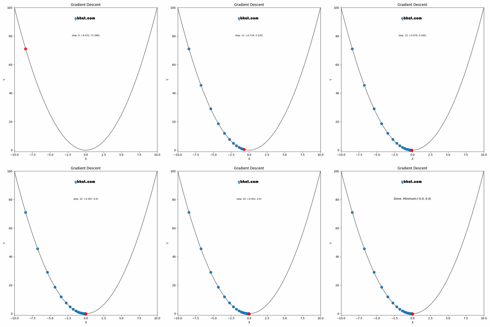
GIF Credit: gbhat.com

Gradient Descent is an optimization algorithm used to minimize the cost function. The cost function \(f(\beta)\) measures how well a model with parameters \(\beta\) fits the data. The goal is to find the values of \(\beta\) that minimize this cost function. In terms of the iterative method, we want to find \(\beta_{k+1}\) and \(\beta_k\) such that \(f(\beta_{k+1})<f(\beta_k)\).

For a small change in \(\beta\), we can approximate \(f(\beta)\) using Taylor series expansion
\[f(\beta_{k+1})=f(\beta_k +\Delta\beta_k)\approx f(\beta_k)+\nabla f(\beta_k)^T \Delta \beta_k+\text{higher-order terms}\]

The update rule for vanilla gradient descent is given by:

\[ \beta_{k+1} = \beta_k - \eta \nabla f(\beta_k) \]

Where:

• \(\beta_k\) is the current estimate of the parameters at iteration \(k\).
• \(\eta\) is the learning rate, a small positive scalar that controls the step size.
• \(\nabla f(\beta_k)\) is the gradient of the cost function \(f\) with respect to \(\beta\) at the current point \(\beta_k\).

The update rule comes from the idea of moving the parameter vector \(\beta\) in the direction that decreases the cost function the most.

1. Gradient: The gradient \(\nabla f(\beta_k)\) represents the direction and magnitude of the steepest ascent of the function \(f\) at the point \(\beta_k\). Since we want to minimize the function, we move in the opposite direction of the gradient.

2. Step Size: The term \(\eta \nabla f(\beta_k)\) scales the gradient by the learning rate \(\eta\), determining how far we move in that direction. If \(\eta\) is too large, the algorithm may overshoot the minimum; if it’s too small, the convergence will be slow.

3. Iterative Update: Starting from an initial guess \(\beta_0\), we repeatedly apply the update rule until the algorithm converges, meaning that the changes in \(\beta_k\) become negligible, and \(\beta_k\) is close to the optimal value \(\beta^*\).

Stochastic Gradient Descent (SGD)

Stochastic Gradient Descent is a variation of the vanilla gradient descent. Instead of computing the gradient using the entire dataset, SGD updates the parameters using only a single data point or a small batch of data points at each iteration. The later one we call it mini batch SGD.

Suppose our cost function is defined as the average over a dataset of size \(n\):

\[ f(\beta) = \frac{1}{n} \sum_{i=1}^{n} f_i(\beta) \]

Where \(f_i(\beta)\) represents the contribution of the \(i\)-th data point to the total cost function. The gradient of the cost function with respect to \(\beta\) is:

\[ \nabla f(\beta) = \frac{1}{n} \sum_{i=1}^{n} \nabla f_i(\beta) \]

Vanilla gradient descent would update the parameters as:

\[ \beta_{k+1} = \beta_k - \eta \nabla f(\beta_k) \]

Instead of using the entire dataset to compute the gradient, SGD approximates the gradient by using only a single data point (or a small batch). The update rule for SGD is:

\[ \beta_{k+1} = \beta_k - \eta \nabla f_{i_k}(\beta_k) \]

Where:

• \(i_k\) is the index of a randomly selected data point at iteration \(k\).
• \(\nabla f_{i_k}(\beta_k)\) is the gradient of the cost function with respect to the parameter \(\beta_k\), evaluated only at the data point indexed by \(i_k\).

Implementation of GD

In 1D

Assume that we have a function \(f(x)=x^2-3x+\frac{13}{4}\) which we want to minimize. Meaning, we want to find \(x\) that minimizes the function.

Next, let’s implement the GD¹

# Define the function
def f(x):
    return x**2-3*x+(13/4)
# Define the gradient function 
def grad_f(x):
    return 2*x-3

# Take a random guess from the domain
local_min = np.random.choice(x)
print('Initial guess: ',local_min )

# Hyper-parameters 
learning_rate = 0.01
training_epochs = 200

model_params = np.zeros((training_epochs,2))
for i in range(training_epochs):
    grad = grad_f(local_min)
    local_min =local_min - learning_rate*grad 
    model_params[i,:] = [local_min, grad]

print('Empirical/estimated local minimum:',local_min)

fig, axs = plt.subplots(1,2, figsize=(8.5,3.8))
for i in range(2):
    axs[i].plot(model_params[:,i],'-')
    axs[i].set_xlabel('Iteration')
    axs[i].set_title(f'Final estimated Min: {local_min:.5f}')
axs[0].set_ylabel('Local Min')
axs[1].set_ylabel('Derivative')
plt.show()

Initial guess:  0.025025025025025016
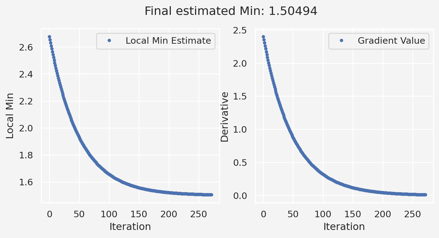
Empirical/estimated local minimum: 1.4740582188953646

Alternatively, if we want to set a tolerance, this is how we set that

# Take a random guess from the domain
local_min = np.random.choice(x)
print('Initial guess:', local_min)

# Hyper-parameters 
learning_rate = 0.01
tolerance = 1e-2  # Stop if gradient is smaller than this value

# Lists to store optimization progress
local_min_vals = []
grad_vals = []
iteration = 0  # Track the number of iterations

# Gradient Descent Loop (Runs until gradient is small enough)
while True:
    grad = grad_f(local_min)
    # Stop when gradient is smaller than tolerance
    if abs(grad) < tolerance:
        print(f"Stopping at iteration {iteration} (grad={grad:.5f})")
        break
    # Update local minimum
    local_min = local_min - learning_rate * grad  
    # Store values
    local_min_vals.append(local_min)
    grad_vals.append(grad)
    iteration += 1  # Increment iteration count

print('Empirical/estimated local minimum:', local_min)

# Convert lists to numpy arrays
local_min_vals = np.array(local_min_vals)
grad_vals = np.array(grad_vals)

# Plot Results
fig, axs = plt.subplots(1, 2, figsize=(8.5, 3.8))

axs[0].plot(local_min_vals, '.', label="Local Min Estimate")
axs[0].set_xlabel('Iteration')
axs[0].set_ylabel('Local Min')
axs[0].legend()

axs[1].plot(grad_vals, '.', label="Gradient Value")
axs[1].set_xlabel('Iteration')
axs[1].set_ylabel('Derivative')
axs[1].legend()

plt.suptitle(f'Final estimated Min: {local_min:.5f}')
plt.show()

Initial guess: 2.701701701701702
Stopping at iteration 272 (grad=0.00987)
Empirical/estimated local minimum: 1.5049350239483508

Parametric variation

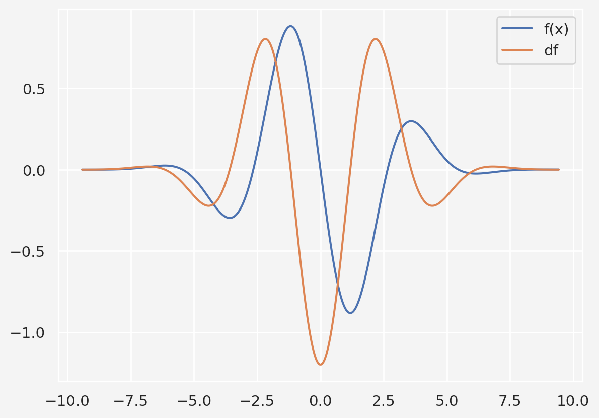
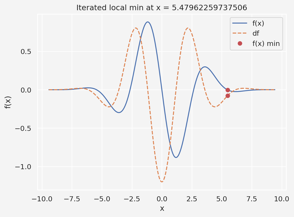
Let’s consider a different problem, \(f(x)=-e^{-\frac{x^2}{10}}(0.2x\cos x+\sin x)\). We want to find the \(x\) values and optimal hyper-parameters that minimizes \(f(x)\).

x = np.linspace(-3*np.pi, 3*np.pi, 400)
y = -np.exp(-(x**2/10))*(0.2*x*np.cos(x)+np.sin(x))

dy = np.exp(-(x**2/10))*((0.04*x**2-1.2)*np.cos(x)+0.4*x*np.sin(x))
plt.plot(x,y, x, dy)
plt.legend(['f(x)','df'])
plt.show()

Clearly, the global minimum is somewhere in between 0 to 2.5, maybe around 1.25. Now let’s apply GD with varying parameters

def f(x):
    f = -np.exp(-(x**2/10))*(0.2*x*np.cos(x)+np.sin(x))
    return f
def df(x):
    ddx_of_f = np.exp(-(x**2/10))*((0.04*x**2-1.2)*np.cos(x)+0.4*x*np.sin(x))
    return ddx_of_f

learning_rate = 0.003
training_epochs = 1000
local_min = np.random.choice(x,1)
print('The chosen initial point: ', local_min)

for i in range(training_epochs):
    grad = df(local_min)
    local_min = local_min - learning_rate*grad 

plt.plot(x,f(x), x, df(x),'--')
plt.plot(local_min, df(local_min),'ro')
plt.plot(local_min, f(local_min),'ro')
plt.xlabel('x')
plt.ylabel('f(x)')
plt.legend(['f(x)','df','f(x) min'])
plt.title('Iterated local min at x = %s'%local_min[0])
plt.show()

The chosen initial point:  [5.17299843]

Now let’s see how we can pick the right initial point

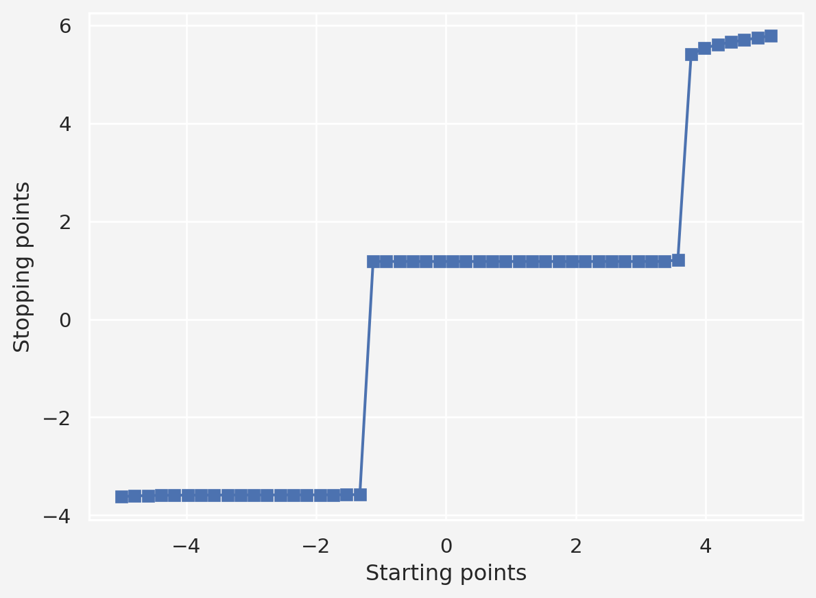
# Vary the starting point 
starting_points = np.linspace(-5,5,50)
stopping_points = np.zeros(len(starting_points))

training_epochs = 1000
learning_rate = 0.01
for idx, local_min in enumerate(starting_points):
    for i in range(training_epochs):
        grad = df(local_min)
        local_min = local_min - learning_rate * grad 
    stopping_points[idx] = local_min
plt.plot(starting_points, stopping_points, 's-')
plt.xlabel('Starting points')
plt.ylabel('Stopping points')
plt.show()

Based on this, if we start with any point roughly between \((-1,3.5)\) we will end up with the global minimum. However, points outside this interval may take the iterative process to other local minima.

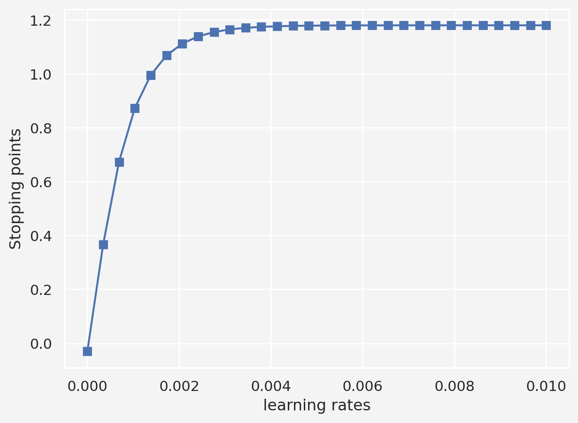
# varying learning rates 
lrs = np.linspace(1e-10, 1e-2, 30)
stopping_points = np.zeros(len(lrs))

training_epochs = 1000

for idx, lr  in enumerate(lrs):
    # fixed initial point 
    local_min = -0.03
    for i in range(training_epochs):
        grad = df(local_min)
        local_min = local_min - lr*grad 
    stopping_points[idx] = local_min
plt.plot(lrs, stopping_points, 's-')
plt.xlabel('learning rates')
plt.ylabel('Stopping points')
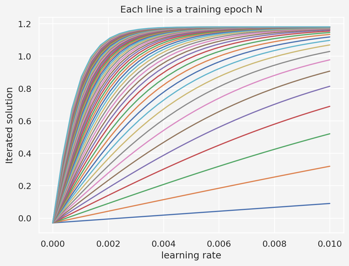
plt.show()

So this suggests that a learning rate between 0.003 to 0.005 is a good start.

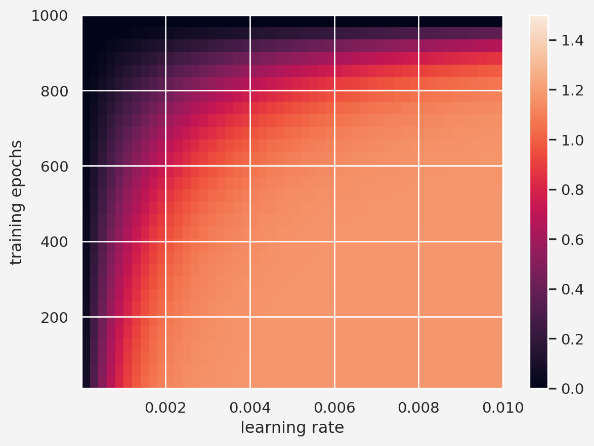
lrs = np.linspace(1e-10, 1e-2, 30)
training_epochs = np.round(np.linspace(10,1000,50))

stopping_points = np.zeros((len(lrs), len(training_epochs)))

for lr_idx, lr in enumerate(lrs):
    for tr_idx, tr_epoch in enumerate(training_epochs):
        local_min = -0.03
        
        for i in range(int(tr_epoch)):
            grad = df(local_min)
            local_min = local_min - lr * grad 

        stopping_points[lr_idx, tr_idx] = local_min
plt.imshow(stopping_points, extent=[lrs[0], lrs[-1],\
     training_epochs[0], training_epochs[-1]], aspect='auto',\
        vmin=0, vmax=1.5)
plt.xlabel('learning rate')
plt.ylabel('training epochs')
plt.colorbar()
plt.show()

We know that the expected minimum at \(x \approx 1.17\) so the color corresponding to this is light. Therefore, if we choose a very small learning rate and/or a larger training epoch then we end up to the darker area which is not a good approximation.

plt.plot(lrs, stopping_points)
plt.xlabel('learning rate')
plt.ylabel('Iterated solution')
plt.title('Each line is a training epoch N')
plt.show

In 2D

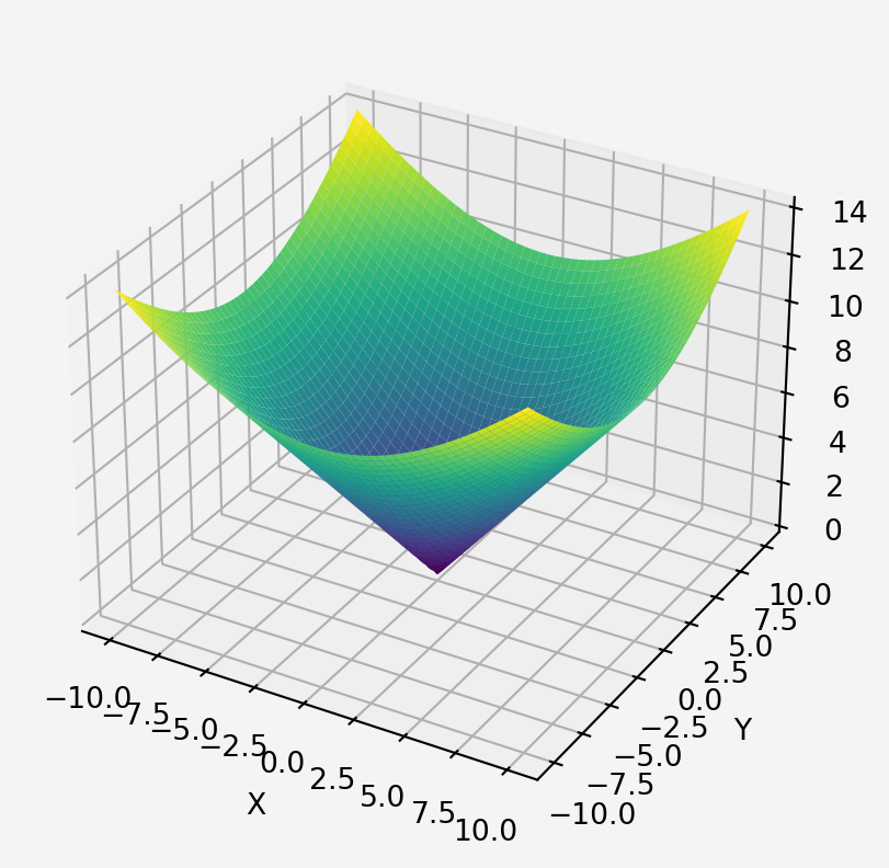
Let’s imagine a hypothetical scenario, Walmart Inc. wants to explore their business in a new twon. They want to have their store in location so that the total distance of the store from all the houses in the neighborhood is the smallest possible. If they have the data of \(n\) houses with corresponding coordinates of the houses, return the optimized location for the store.

The Euclidean distance between two points \((x_1,y_1)\) and \((x_2,y_2)\) is given by
\[d=\sqrt{(x_1-x_2)^2+(y_1-y_2)}\]

Assume that \(P=(x,y)\) is the coordinate of Walmart. So for a total of \(n\) such points the total distance \(D\) from the point \(P\) is a function of two variable \(x\) and \(y\) of the following form

\[D=f(x,y)=\sum_{i=1}^{n}\sqrt{(x-x_i)^2+(y-y_i)^2}\]

import plotly.offline as iplot
import plotly as py
py.offline.init_notebook_mode(connected=True)
import plotly.graph_objects as go


def f(x,y, c, d):
    return np.sqrt((x-c)**2+(y-d)**2)

x = np.linspace(-10,10, 400)
y = np.linspace(-10,10, 400)
x, y = np.meshgrid(x,y)

c, d = 0,0

z = f(x, y, c, d)

fig = go.Figure(data=[go.Surface(z=z, x=x, y=y)])
fig.update_layout(
    title='3D plot',
    scene=dict(
        xaxis_title = 'x',
        yaxis_title = 'y',
        zaxis_title = 'z'
    )
)

fig.show()

all we need to do is to minimize the function \(f(x,y)\) and to do that we need to calculate the gradient vector which is the partial derivative of \(f(x,y)\) with respect to \(x\) and \(y\). So,

\[\begin{align*} \frac{\partial f}{\partial x}& = \sum_{i=1}^{n} \frac{x-x_i}{\sqrt{(x-x_i)^2+(y-y_i)^2}}\\ \frac{\partial f}{\partial y}& = \sum_{i=1}^{n} \frac{y-y_i}{\sqrt{(x-x_i)^2+(y-y_i)^2}}\\ & \\ \implies \nabla f(x,y) &= \begin{bmatrix}\frac{\partial f}{\partial x}\\\frac{\partial f}{\partial y}\end{bmatrix} \end{align*}\]

Then the algorithm

\[\begin{align*} \begin{bmatrix}x_{i+1}\\y_{i+1}\end{bmatrix}&= \begin{bmatrix}x_{i}\\y_{i}\end{bmatrix} - \eta_i \begin{bmatrix}\frac{\partial f}{\partial x}|_{x_i}\\\frac{\partial f}{\partial y}|_{y_i}\end{bmatrix} \end{align*}\]

where, the \(\eta\) is the step size or learning rate that scales the size of the move towards the opposite of the gradient direction.

Next, how do we control the numerical stability of the algorithm? We need to decrease the step size at each iteration which. This is called the rate of decay. We also need a termination factor or tolerance level that determines if we can stop the iteration. Sometimes, for a deep down convex function, the process oscillates back and forth around a range of values. In this case, applying a damping factor increases the chance for a smooth convergence.

import numpy as np
import matplotlib.pyplot as plt
import math

class GDdistanceMin:
    def __init__(self, step_size=1, decay_rate=0.99, tolerance=1e-7, damping_rate=0.75, points=[]):
        self.step_size = step_size
        self.decay_rate = decay_rate
        self.tolerance = tolerance
        self.damping_rate = damping_rate
        self.points = points
        self.x = sum(x for x, y in points) / len(points)  # Initialization
        self.y = sum(y for x, y in points) / len(points)  # Initialization
        self.x_updates = []
        self.y_updates = []

    def _partial_derivative_x(self, x, y):
        grad_x = 0
        for xi, yi in self.points:
            if x != xi or y != yi:
                grad_x += (x - xi) / math.sqrt((x - xi)**2 + (y - yi)**2)
        return grad_x

    def _partial_derivative_y(self, x, y):
        grad_y = 0
        for xi, yi in self.points:
            if x != xi or y != yi:
                grad_y += (y - yi) / math.sqrt((x - xi)**2 + (y - yi)**2)
        return grad_y

    def gradient_descent(self):
        dx, dy = 0, 0
        while self.step_size > self.tolerance:
            dx = self._partial_derivative_x(self.x, self.y) + self.damping_rate * dx 
            dy = self._partial_derivative_y(self.x, self.y) + self.damping_rate * dy 
            self.x -= self.step_size * dx 
            self.x_updates.append(self.x)
            self.y -= self.step_size * dy 
            self.y_updates.append(self.y)
            self.step_size *= self.decay_rate
        return (self.x, self.y)

def f(x, y, c, d):
    return np.sqrt((x - c)**2 + (y - d)**2)

# Define points
points = [(1, 3), (-2, 4), (3, 4), (-2, 1), (9, 2), (-5, 2)]
gd_min = GDdistanceMin(points=points)
min_pt = gd_min.gradient_descent()
xs = gd_min.x_updates
ys = gd_min.y_updates
print("Minimum point:", min_pt)

c, d = min_pt

# Create a grid for plotting
x = np.linspace(-10, 10, 400)
y = np.linspace(-10, 10, 400)
x_grid, y_grid = np.meshgrid(x, y)
z = f(x_grid, y_grid, c, d)

# Calculate z values for the updates
zs = [f(xi, yi, c, d) for xi, yi in zip(xs, ys)]

# Plotting
fig = plt.figure()
ax = fig.add_subplot(111, projection='3d')
ax.plot_surface(x_grid, y_grid, z, cmap='viridis', alpha=0.6)
ax.scatter(xs, ys, zs, color='red', s=50, label="Updates", marker='o')
ax.set_xlabel('X')
ax.set_ylabel('Y')
ax.set_zlabel('Z')
plt.gca().set_facecolor('#f4f4f4') 
plt.gcf().patch.set_facecolor('#f4f4f4')
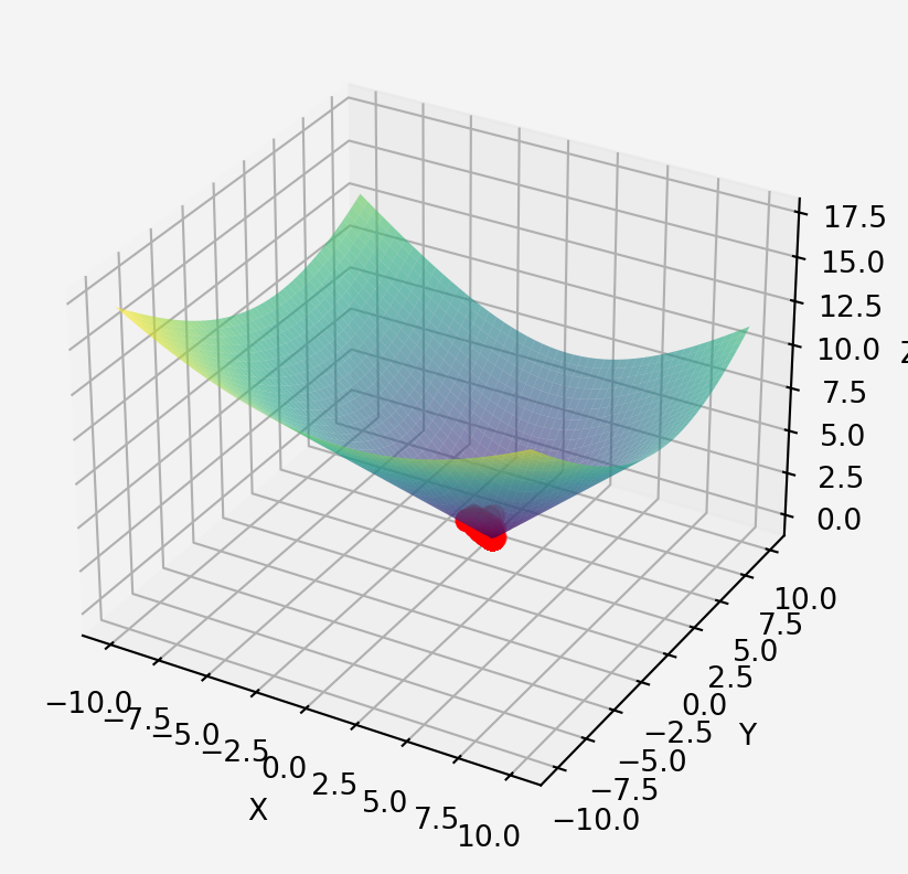
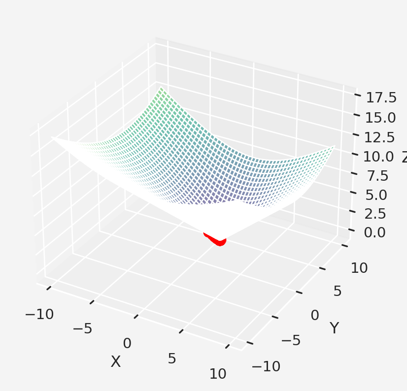
plt.show()

Minimum point: (0.9999997458022071, 2.9999999769909707)

Different approach²

import sympy as sym 
sym.init_printing()
from IPython.display import display, Math
from matplotlib_inline.backend_inline import set_matplotlib_formats
set_matplotlib_formats('svg') 


def distance_function(x,y,c,d):
    x,y = np.meshgrid(x,y)
    z = np.sqrt((x-c)**2+(y-d)**2)
    return z

c,d = 0,0
x = np.linspace(-5,5, 400)
y = np.linspace(-5,5, 400)
z = distance_function(x,y,c,d)

plt.imshow(z, extent=[x[0],x[-1], y[0],y[-1]],vmin=-5, vmax=5, origin='lower')
plt.show()

So, the minimum is in the center of the deep color area. Let’s compute the derivatives using sympy library

sx, sy = sym.symbols('sx,sy')
sz = sym.sqrt((sx-c)**2+(sy-d)**2)

df_sx = sym.lambdify((sx,sy), sym.diff(sz, sx), 'sympy')
df_sy = sym.lambdify((sx,sy), sym.diff(sz, sy), 'sympy')

display(Math(f"\\frac{{\\partial f}}{{\\partial x}}={sym.latex(sym.diff(sz,sx))}\
     \\text{{ and }}  \\frac{{\\partial f}}{{\\partial x}}\\mid_{{(1,1)}} = {df_sx(1,1).evalf()}"))
display(Math(f"\\frac{{\\partial f}}{{\\partial y}}={sym.latex(sym.diff(sz,sy))} \
     \\text{{ and }}  \\frac{{\\partial f}}{{\\partial y}}\\mid_{{(1,1)}} = {df_sy(1,1).evalf()}"))

\(\displaystyle \frac{\partial f}{\partial x}=\frac{sx}{\sqrt{sx^{2} + sy^{2}}} \text{ and } \frac{\partial f}{\partial x}\mid_{(1,1)} = 0.707106781186548\)

\(\displaystyle \frac{\partial f}{\partial y}=\frac{sy}{\sqrt{sx^{2} + sy^{2}}} \text{ and } \frac{\partial f}{\partial y}\mid_{(1,1)} = 0.707106781186548\)

Now let’s implement the GD

# Let's pick a random starting point(uniformly distributed between -2 and 2)
local_min = np.random.rand(2)*4-2
start_point = local_min[:] # make a copy

learning_rate = 0.01
training_epochs = 1000

trajectory = np.zeros((training_epochs,2))

for i in range(training_epochs):
    grad = np.array([
        df_sx(local_min[0],local_min[1]).evalf(),
        df_sy(local_min[0],local_min[1]).evalf()
    ])
    local_min = local_min - learning_rate*grad
    trajectory[i,:] = local_min

print('Starting point ',start_point)
print('Local min found ',local_min)

plt.imshow(z, extent=[x[0],x[-1], y[0],y[-1]],vmin=-5, vmax=5, origin='lower')
plt.plot(start_point[0], start_point[1], 'bs')
plt.plot(local_min[0],local_min[1],'rs')
plt.plot(trajectory[:,0],trajectory[:,1], 'b', linewidth=3)
plt.legend(['random start', 'local min'])
plt.colorbar()
plt.show()

Starting point  [1.22754924 0.7182846 ]
Local min found  [0.00194648371310253 0.00113895983415082]

Implementation of SGD

Personally, I think this webpage is one of the best resources for learning how to implement SGD.

---

Share on

You may also like

Footnotes

1. The implementation is taken from the the Udemy course A Deep Understanding of Deep Learning

2. The implementation is taken from the the Udemy course A Deep Understanding of Deep Learning