Bayesian Inference in Machine Learning: Part 1
Introduction
 Bayesian inference is a powerful statistical method that applies the principles of Bayes’s theorem to update the probability of a hypothesis as more evidence or information becomes available. It is widely used in various fields including machine learning, to make predictions and decisions under uncertainty.
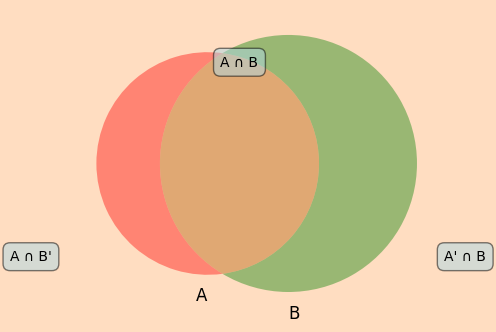
Bayes’s theorem is a fundamental result in probability theory that relates the conditional and marginal probabilities of random events. Mathematically,
\[\mathbb{P}(A|B)=\frac{\mathbb{P}(B|A)\mathbb{P}(A)}{\mathbb{P}(B)}\hspace{4mm} \implies \mathbb{P}(A|B) \propto \mathbb{P}(B|A)\mathbb{P}(A)\]
where, \(A\) and \(B\) are events and \(\mathbb{P}(B)\ne 0\).
- \(\mathbb{P}(A|B)\) is a conditional probability which states the probability of occuring the event \(A\) when the event \(B\) is given or true. The other name of this quantity is called posterior probability of \(A\) given the event \(B\) or simply, posterior distribution.
- \(\mathbb{P}(B|A)\) is a conditional probability which states the probability of occuring the event \(B\) when the event \(A\) is given or true. In other terms, \(\mathbb{P}(B|A)\) is the likelihood: the probability of evidence \(B\) given that \(A\) is true.
- \(\mathbb{P}(A)\) or \(\mathbb{P}(B)\) are the probabilities of occuring \(A\) and \(B\) respectively, without any dependence on each other. \(\mathbb{P}(A)\) is called the prior probability or prior distribution and \(\mathbb{P}(B)\) is called the marginal likelihood or marginal probabilities.
Example 1
Consider a medical example where we want to diagnose a disease based on a test result. Let:
- \(D\) be the event that a patient has the disease.
- \(T\) be the event that the test result is positive.
We are interested in finding the probability that a patient has the disease given a positive test result, \(\mathbb{P}(D|T)\).
Given:
- \(\mathbb{P}(T|D) = 0.99\) (the probability of a positive test result given the patient has the disease).
- \(\mathbb{P}(D) = 0.01\) (the prior probability of the disease).
- \(\mathbb{P}(T|D') = 0.05\) (the probability of a positive test result given the patient does not have the disease).
First, we need to calculate the marginal likelihood \(P(T)\): \[\begin{align*} \mathbb{P}(T) &= \mathbb{P}(T|D) \cdot \mathbb{P}(D) + \mathbb{P}(T|D') \cdot \mathbb{P}(D') \\ \mathbb{P}(T) &= 0.99 \cdot 0.01 + 0.05 \cdot 0.99\\ \mathbb{P}(T) &= 0.0099 + 0.0495 \\ \mathbb{P}(T) &= 0.0594 \end{align*}\]
Now, we can apply Bayes’s theorem:
\[\begin{align*}
\mathbb{P}(D|T) &= \frac{\mathbb{P}(T|D) \cdot \mathbb{P}(D)}{\mathbb{P}(T)}\\
\mathbb{P}(D|T) &= \frac{0.99 \cdot 0.01}{0.0594}\\
\mathbb{P}(D|T) &\approx 0.1667
\end{align*}\]
So, the probability that the patient has the disease given a positive test result is approximately \(16.67\%\).
Example 2
 Assume that you are in a restuarant and you ordered a plate of 3 pancakes. The chef made three pancakes with one in perfect condition, that is not burnt in any side, one with one side burnt, and the last one burnt in both sides. The waiter wanted to stack the pancakes so that the burnt side does not show up when served. However, the chef recommended not to hide the burnt side and asked her to stack the pancakes randomly. What is the likelyhood that the fully burnt pancake will be on the top?
To solve this problem, we can use Bayesian approach. We denote the event \(X\) as the pancake without any burnt, \(Y\) with one side burnt, and \(Z\) both side burnt. Then we have the following conditional probabilities
\[\begin{align*} \mathbb{P}(\text{top-burnt} | X)&=0\\ \mathbb{P}(\text{top-burnt} | Y)&=\frac{1}{2}\\ \mathbb{P}(\text{top-burnt} | Z)&=1\\ \end{align*}\]
The probability of picking a pancake irrespective of their burnt condition is \(\frac{1}{3}\). So,
\[\begin{equation}
\mathbb{P}(X)=\mathbb{P}(Y)=\mathbb{P}(Z)=\frac{1}{3}
\end{equation}\]
The marginal probability of having burnt side in the top position
\[\begin{align*}
\mathbb{P}(\text{top-burnt})&=\mathbb{P}(\text{top-burnt}|X)\mathbb{P}(X)+\mathbb{P}(\text{top-burnt}|Y)\mathbb{P}(Y)+\mathbb{P}(\text{top-burnt}|Z)\mathbb{P}(Z)\\
&=0\cdot \frac{1}{3}+\frac{1}{2}\cdot\frac{1}{3}+1\cdot\frac{1}{3}\\
&=\frac{1}{2}
\end{align*}\]
Now, we can only have a burnt side on top if either \(Z\) is placed in the top or the burnt side of \(Y\) is placed in the top. \[\begin{align*} \mathbb{P}(Y|\text{top-burnt})&=\frac{\mathbb{P}(\text{top-burnt}|Y)\mathbb{P}(Y)}{\mathbb{P}(\text{top-burnt})}\\ &=\frac{\mathbb{P}(\text{top-burnt}|Y)\mathbb{P}(Y)}{\mathbb{P}(\text{top-burnt}|X)\mathbb{P}(X)+\mathbb{P}(\text{top-burnt}|Y)\mathbb{P}(Y)+\mathbb{P}(\text{top-burnt}|Z)\mathbb{P}(Z)}\\ &=\frac{\frac{1}{2}\cdot\frac{1}{3}}{\frac{1}{2}}=\frac{1}{3}\\ \mathbb{P}(Z|\text{top-burnt})&=\frac{\mathbb{P}(\text{top-burnt}|Z)\mathbb{P}(Z)}{\mathbb{P}(\text{top-burnt})}\\ &=\frac{\mathbb{P}(\text{top-burnt}|Z)\mathbb{P}(Z)}{\mathbb{P}(\text{top-burnt}|X)\mathbb{P}(X)+\mathbb{P}(\text{top-burnt}|Y)\mathbb{P}(Y)+\mathbb{P}(\text{top-burnt}|Z)\mathbb{P}(Z)}\\ &=\frac{\frac{1}{3}}{\frac{1}{2}}=\frac{2}{3} \end{align*}\]
So the probability of having the fully burnt pancake on the top is \(\frac{2}{3}\).
Why Bayesian Inference in Machine Learning?
Bayesian inference plays a crucial role in machine learning, particularly in areas involving uncertainty and probabilistic reasoning. It allows us to incorporate prior knowledge and update beliefs based on new data, which is especially useful in the following applications:
Bayesian Networks
Bayesian networks are graphical models that represent the probabilistic relationships among a set of variables. Each node in the network represents a random variable, and the edges represent conditional dependencies. Bayesian networks are used for various tasks such as classification, prediction, and anomaly detection.
Bayesian Regression
Bayesian regression extends linear regression by incorporating prior distributions on the model parameters. This approach provides a probabilistic framework for regression analysis, allowing for uncertainty in the parameter estimates. The posterior distribution of the parameters is computed using Bayes’s theorem, and predictions are made by averaging over this distribution.
Sampling Methods
In Bayesian inference, exact computation of the posterior distribution is often intractable. Therefore, sampling methods such as Markov Chain Monte Carlo (MCMC) and Variational Inference are used to approximate the posterior distribution. These methods generate samples from the posterior distribution, allowing us to estimate various statistical properties and make inferences.
Markov Chain Monte Carlo (MCMC)
MCMC methods generate a sequence of samples from the posterior distribution by constructing a Markov chain that has the desired distribution as its equilibrium distribution. Common MCMC algorithms include the Underdamped and Overdamped Langevin dynamics, Metropolis-Hastings algorithm and the Gibbs sampler.
Example: Metropolis-Hastings Algorithm
Consider a posterior distribution \(P(\theta|D)\) where \(\theta\) represents the model parameters and \(D\) represents the data. The Metropolis-Hastings algorithm proceeds as follows:
- Initialize the parameters \(\theta_0\).
- For \(t = 1\) to \(T\):
- Propose a new state \(\theta'\) from a proposal distribution \(Q(\theta'|\theta_t)\).
- Compute the acceptance ratio \(\alpha = \frac{P(\theta'|D) \cdot Q(\theta_t|\theta')}{P(\theta_t|D) \cdot Q(\theta'|\theta_t)}\).
- Accept the new state with probability \(\min(1, \alpha)\). If accepted, set \(\theta_{t+1} = \theta'\); otherwise, set \(\theta_{t+1} = \theta_t\).
The samples \(\theta_1, \theta_2, \ldots, \theta_T\) form a Markov chain whose stationary distribution is the posterior distribution \(P(\theta|D)\).
Bayesian Inference in Neural Networks
Bayesian methods are also applied to neural networks, resulting in Bayesian Neural Networks (BNNs). BNNs incorporate uncertainty in the network weights by placing a prior distribution over them and using Bayes’s theorem to update this distribution based on the observed data. This allows BNNs to provide not only point estimates but also uncertainty estimates for their predictions.
In the next parts, we will talk about different applications of the Bayesian inferences, specifically, sampling problem using Langevin dynamics.
Reference
Share on
You may also like
Citation
@online{islam2024,
  author = {Islam, Rafiq},
  title = {Bayesian {Inference} in {Machine} {Learning:} {Part} 1},
  date = {2024-07-28},
  url = {https://mrislambd.github.io/jobandintern/bayesianinference/},
  langid = {en}
}


