from mywebstyle import plot_styleimport matplotlib.pyplot as pltimport seaborn as snsimport numpy as npimport pandas as pdimport kaggle'#f4f4f4' )= pd.read_csv('lending_club_loan_two.csv' )= loandata.iloc[:, :13 ]
Warning: Your Kaggle API key is readable by other users on this system! To fix this, you can run 'chmod 600 /Users/macpc/.kaggle/kaggle.json'
0
10000
36 months
11.44
329.48
B
B4
Marketing
10+ years
RENT
117000.0
Not Verified
Jan-15
Fully Paid
1
8000
36 months
11.99
265.68
B
B5
Credit analyst
4 years
MORTGAGE
65000.0
Not Verified
Jan-15
Fully Paid
2
15600
36 months
10.49
506.97
B
B3
Statistician
< 1 year
RENT
43057.0
Source Verified
Jan-15
Fully Paid
3
7200
36 months
6.49
220.65
A
A2
Client Advocate
6 years
RENT
54000.0
Not Verified
Nov-14
Fully Paid
4
24375
60 months
17.27
609.33
C
C5
Destiny Management Inc.
9 years
MORTGAGE
55000.0
Verified
Apr-13
Charged Off
= loandata.iloc[:, 13 :]
0
vacation
Vacation
26.24
Jun-90
16
0
36369
41.8
25
w
INDIVIDUAL
0.0
0.0
0174 Michelle Gateway\r\nMendozaberg, OK 22690
1
debt_consolidation
Debt consolidation
22.05
Jul-04
17
0
20131
53.3
27
f
INDIVIDUAL
3.0
0.0
1076 Carney Fort Apt. 347\r\nLoganmouth, SD 05113
2
credit_card
Credit card refinancing
12.79
Aug-07
13
0
11987
92.2
26
f
INDIVIDUAL
0.0
0.0
87025 Mark Dale Apt. 269\r\nNew Sabrina, WV 05113
3
credit_card
Credit card refinancing
2.60
Sep-06
6
0
5472
21.5
13
f
INDIVIDUAL
0.0
0.0
823 Reid Ford\r\nDelacruzside, MA 00813
4
credit_card
Credit Card Refinance
33.95
Mar-99
13
0
24584
69.8
43
f
INDIVIDUAL
1.0
0.0
679 Luna Roads\r\nGreggshire, VA 11650
<class 'pandas.core.frame.DataFrame'>
RangeIndex: 395900 entries, 0 to 395899
Data columns (total 27 columns):
 #   Column                Non-Null Count   Dtype
---  ------                --------------   -----
 0   loan_amnt             395900 non-null  int64
 1   term                  395900 non-null  object
 2   int_rate              395900 non-null  float64
 3   installment           395900 non-null  float64
 4   grade                 395900 non-null  object
 5   sub_grade             395900 non-null  object
 6   emp_title             372982 non-null  object
 7   emp_length            377608 non-null  object
 8   home_ownership        395900 non-null  object
 9   annual_inc            395900 non-null  float64
 10  verification_status   395900 non-null  object
 11  issue_d               395900 non-null  object
 12  loan_status           395900 non-null  object
 13  purpose               395900 non-null  object
 14  title                 394145 non-null  object
 15  dti                   395900 non-null  float64
 16  earliest_cr_line      395900 non-null  object
 17  open_acc              395900 non-null  int64
 18  pub_rec               395900 non-null  int64
 19  revol_bal             395900 non-null  int64
 20  revol_util            395624 non-null  float64
 21  total_acc             395900 non-null  int64
 22  initial_list_status   395900 non-null  object
 23  application_type      395900 non-null  object
 24  mort_acc              358117 non-null  float64
 25  pub_rec_bankruptcies  395365 non-null  float64
 26  address               395900 non-null  object
dtypes: float64(7), int64(5), object(15)
memory usage: 81.6+ MB
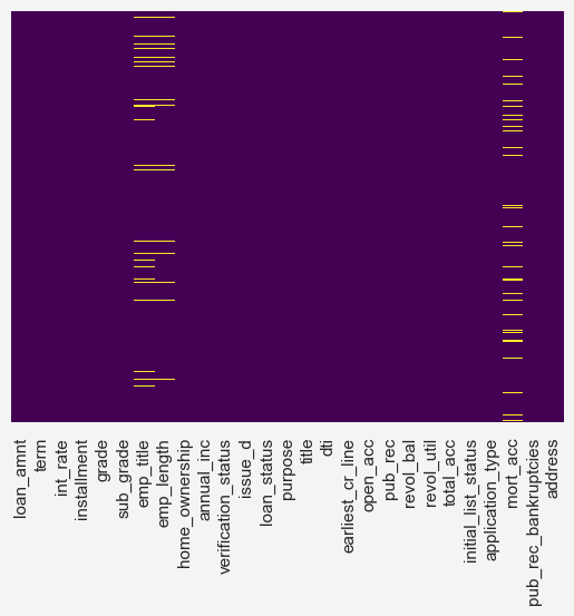
= False , cbar= False , cmap= 'viridis' )
loan_amnt
395900.0
14114.249305
8357.637338
500.00
8000.00
12000.00
20000.00
40000.00
int_rate
395900.0
13.639385
4.472112
5.32
10.49
13.33
16.49
30.99
installment
395900.0
431.859947
250.733444
16.08
250.33
375.43
567.30
1533.81
annual_inc
395900.0
74206.819251
61645.032777
0.00
45000.00
64000.00
90000.00
8706582.00
dti
395900.0
17.379187
18.021550
0.00
11.28
16.91
22.98
9999.00
open_acc
395900.0
11.311081
5.137591
0.00
8.00
10.00
14.00
90.00
pub_rec
395900.0
0.178204
0.530716
0.00
0.00
0.00
0.00
86.00
revol_bal
395900.0
15844.331435
20589.846553
0.00
6026.00
11181.00
19620.00
1743266.00
revol_util
395624.0
53.793449
24.452575
0.00
35.80
54.80
72.90
892.30
total_acc
395900.0
25.414622
11.887279
2.00
17.00
24.00
32.00
151.00
mort_acc
358117.0
1.814091
2.148006
0.00
0.00
1.00
3.00
34.00
pub_rec_bankruptcies
395365.0
0.121647
0.356176
0.00
0.00
0.00
0.00
8.00
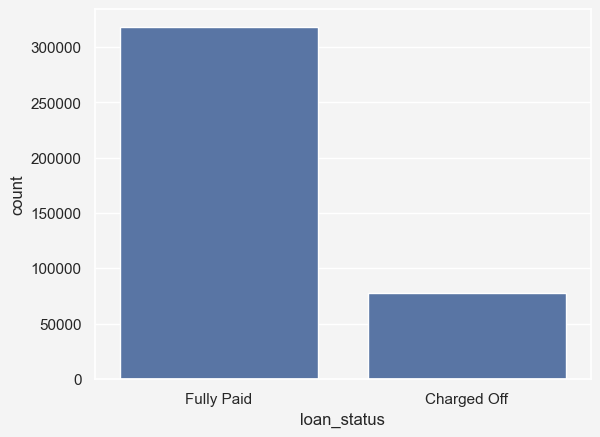
= 'loan_status' , data= loandata)= np.round (len (loandata[loandata['loan_status' ] == 'Fully Paid' ])/ len (loandata)* 100 , 2 = np.round (len (loandata[loandata['loan_status' ] == 'Charged Off' ]) / len (loandata)* 100 , 2
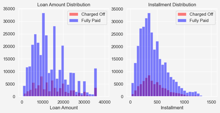
= plt.figure(figsize= (9 , 4 ))= fig.add_subplot(121 )'loan_status' ] == 'Charged Off' ]['loan_amnt' ].hist(= 0.5 , color= 'red' , bins= 30 , ax= ax1,= 'Charged Off' 'loan_status' ] == 'Fully Paid' ]['loan_amnt' ].hist(= 0.5 , color= 'blue' , bins= 30 , ax= ax1,= 'Fully Paid' 'Loan Amount Distribution' )'Loan Amount' )= fig.add_subplot(122 )'loan_status' ] == 'Charged Off' ]['installment' ].hist(= 0.5 , color= 'red' , bins= 30 , ax= ax2,= 'Charged Off' 'loan_status' ] == 'Fully Paid' ]['installment' ].hist(= 0.5 , color= 'blue' , bins= 30 , ax= ax2,= 'Fully Paid' 'Installment Distribution' )'Installment' )
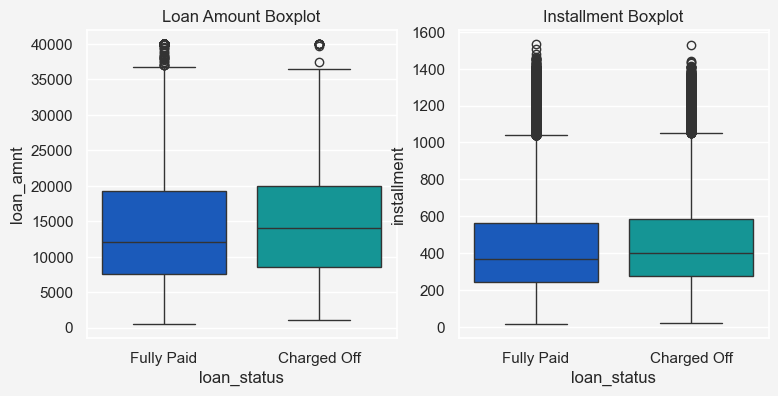
= plt.figure(figsize= (8.8 , 4 ))= fig.add_subplot(121 )= 'loan_status' , y= 'loan_amnt' , hue= 'loan_status' ,= loandata, ax= ax1, palette= 'winter' 'Loan Amount Boxplot' )= fig.add_subplot(122 )= 'loan_status' , y= 'installment' , hue= 'loan_status' ,= loandata, ax= ax2, palette= 'winter' 'Installment Boxplot' )
Text(0.5, 1.0, 'Installment Boxplot')
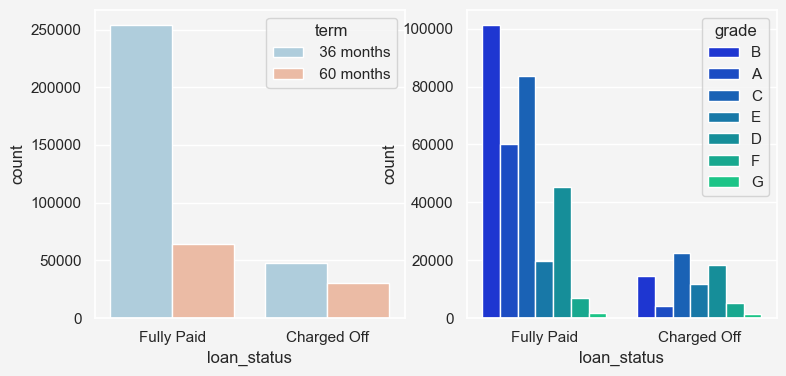
= plt.figure(figsize= (8.8 , 4 ))= fig.add_subplot(121 )= 'loan_status' ,= 'term' , data= loandata,= 'RdBu_r' , ax= ax1= fig.add_subplot(122 )= 'loan_status' ,= 'grade' , data= loandata,= 'winter' , ax= ax2
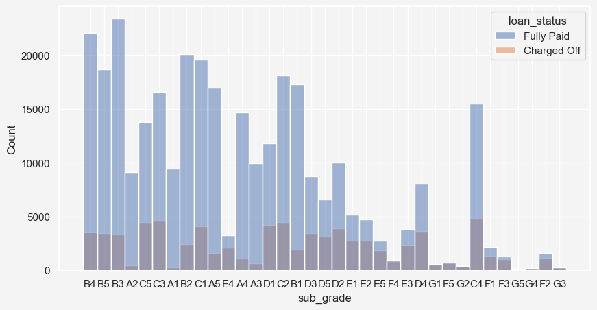
= plt.subplots(figsize= (10 , 5 ))= 'sub_grade' , hue= 'loan_status' , data= loandata, ax= ax)
'emp_title' ] = loandata['emp_title' ].str .lower()25 ]
emp_title
manager                     5635
teacher                     5426
registered nurse            2626
supervisor                  2589
sales                       2381
driver                      2306
owner                       2200
rn                          2072
project manager             1776
office manager              1638
general manager             1460
truck driver                1288
director                    1192
engineer                    1187
police officer              1041
vice president               961
sales manager                961
operations manager           960
store manager                941
president                    877
administrative assistant     865
accountant                   845
account manager              845
technician                   839
mechanic                     753
Name: count, dtype: int64
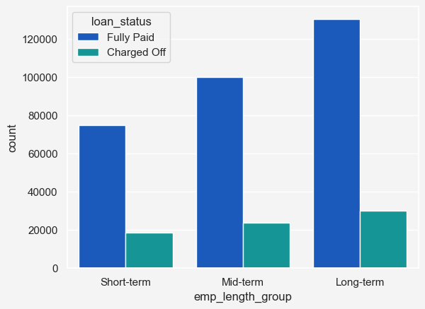
'future.no_silent_downcasting' , True )'emp_length' ] = loandata['emp_length' ].replace({'< 1 year' : 0 ,'1 year' : 1 ,'2 years' : 2 ,'3 years' : 3 ,'4 years' : 4 ,'5 years' : 5 ,'6 years' : 6 ,'7 years' : 7 ,'8 years' : 8 ,'9 years' : 9 ,'10+ years' : 10 = False )'emp_length_group' ] = pd.cut('emp_length' ],= [- 1 , 2 , 7 , 10 ], # Bins: <3 years, 3-7 years, > 7 years = ['Short-term' , 'Mid-term' , 'Long-term' ]= 'emp_length_group' ,= 'loan_status' ,= loandata,= 'winter' ,= 'count'
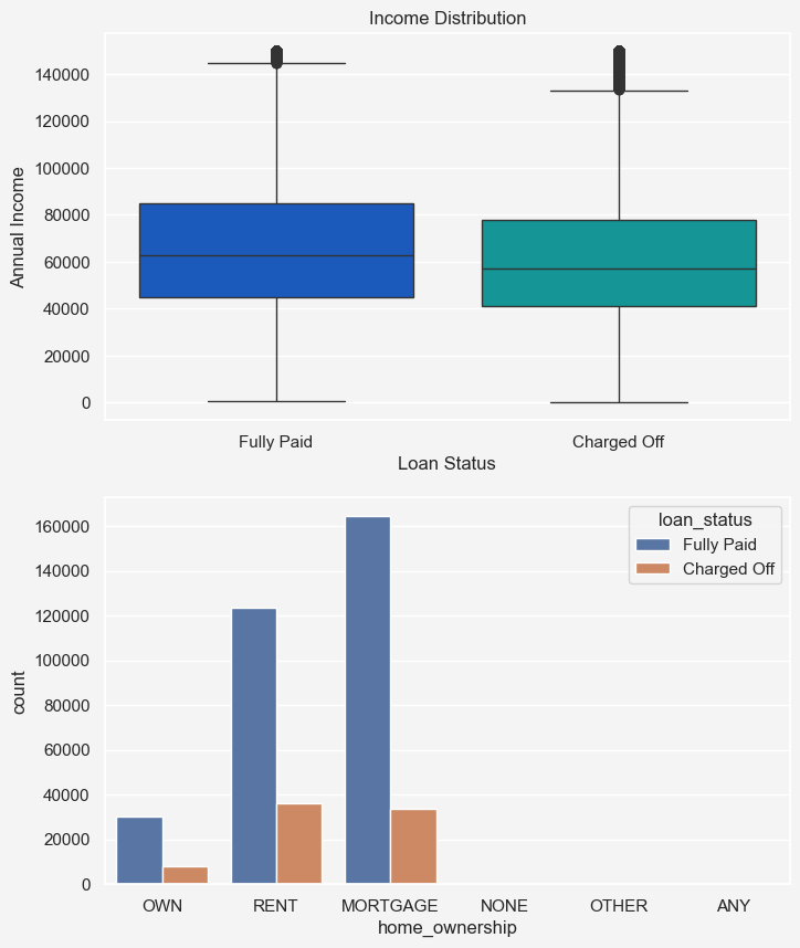
= plt.figure(figsize= (8 , 10 ))= fig.add_subplot(211 )= loandata['annual_inc' ].quantile(0.95 )= loandata[loandata['annual_inc' ] <= annual_income_threshod]= 'loan_status' , y= 'annual_inc' ,= 'loan_status' , palette= 'winter' ,= filtered_income, ax= ax1'Income Distribution' )'Loan Status' )'Annual Income' )= fig.add_subplot(212 )= 'home_ownership' , hue= 'loan_status' ,= loandata, ax= ax2
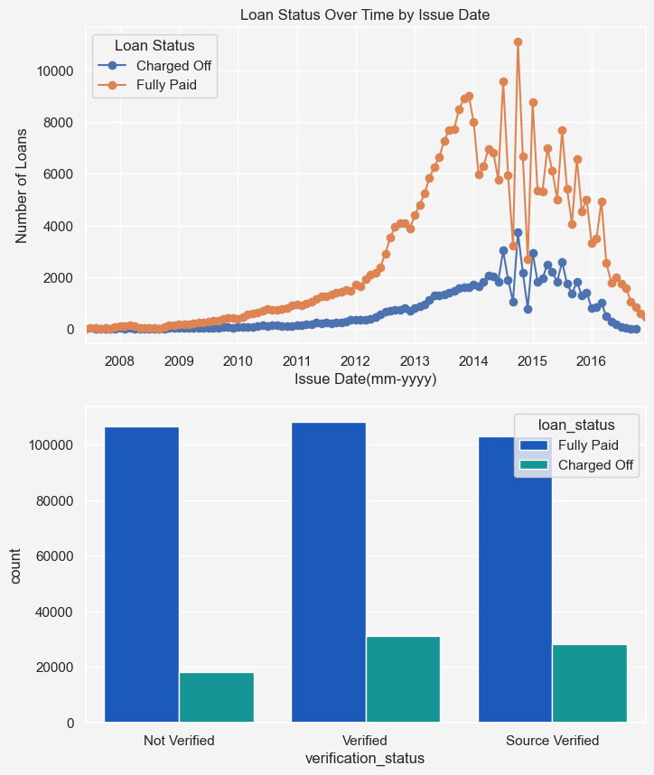
'issue_d' ] = pd.to_datetime('issue_d' ], format = '%b-%y' = loandata.sort_values('issue_d' )= loandata.groupby('issue_d' , 'loan_status' ]).size().unstack()= plt.figure(figsize= (8 , 10 ))= fig.add_subplot(211 )= 'line' , marker= 'o' , ax= ax1'Loan Status Over Time by Issue Date' )'Issue Date(mm-yyyy)' )'Number of Loans' )= 'Loan Status' )= fig.add_subplot(212 )= 'verification_status' , hue= 'loan_status' ,= loandata, palette= 'winter' , ax= ax2
'purpose' ].value_counts()
purpose
debt_consolidation    234420
credit_card            82998
home_improvement       24024
other                  21177
major_purchase          8788
small_business          5701
car                     4696
medical                 4194
moving                  2853
vacation                2452
house                   2201
wedding                 1811
renewable_energy         328
educational              257
Name: count, dtype: int64
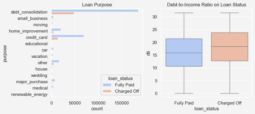
= plt.figure(figsize= (9 , 4 ))= fig.add_subplot(121 )= 'purpose' , hue= 'loan_status' ,= loandata, palette= 'coolwarm' 'Loan Purpose' )= fig.add_subplot(122 )= loandata['dti' ].quantile(0.95 )= loandata[loandata['dti' ] <= dti_threshold]= 'loan_status' , y= 'dti' ,= 'loan_status' , data= filtereddata,= 'coolwarm' , ax= ax2'Debt-to-Income Ratio on Loan Status' )
Text(0.5, 1.0, 'Debt-to-Income Ratio on Loan Status')
Insights: From the purpose column, we see that most of the loans that were charged off were used to make debt consolidation. Therefore, debt consolidation may have been a significant factor when a loan is charged off. Another insight we obtain from the debt-to-income ratio is that the charged off loans have higher dti ratio
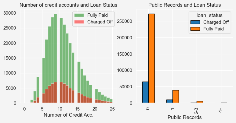
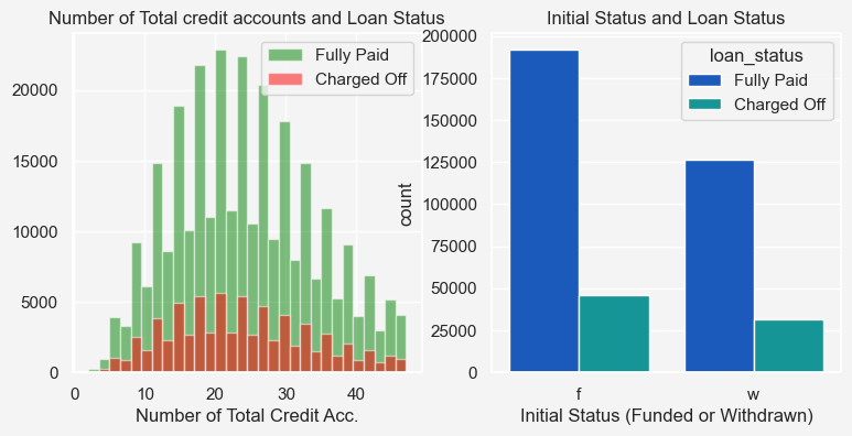
= plt.figure(figsize= (9 , 4 ))= fig.add_subplot(121 )= loandata['open_acc' ].quantile(0.98 )= loandata[loandata['open_acc' ]<= filtered_open_account_threshold]'loan_status' ] == 'Fully Paid' ]['open_acc' ].hist(= 0.5 , color= 'green' , bins= 30 , label= 'Fully Paid' , ax= ax1'loan_status' ] == 'Charged Off' ]['open_acc' ].hist(= 0.5 , color= 'red' , bins= 30 , label= 'Charged Off' , ax= ax1'Number of Credit Acc.' )'Number of credit accounts and Loan Status' )'pub_rec_group' ] = pd.cut('pub_rec' ], bins= [- 1 , 0 , 1 , 3 , loandata['pub_rec' ].max ()],= ['0' , '1' , '2-3' , '4+' ]= loandata.groupby('pub_rec_group' , 'loan_status' ], observed= False = fig.add_subplot(122 )= 'bar' , stacked= False , edgecolor= 'black' ,= ['#1f77b4' , '#ff7f0e' ], ax= ax2'Public Records and Loan Status' )'Public Records' )
Text(0.5, 0, 'Public Records')
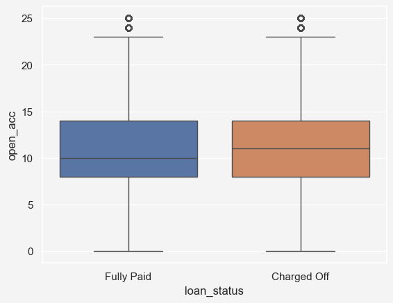
= 'open_acc' , x= 'loan_status' ,= 'loan_status' ,= filtered_open_account
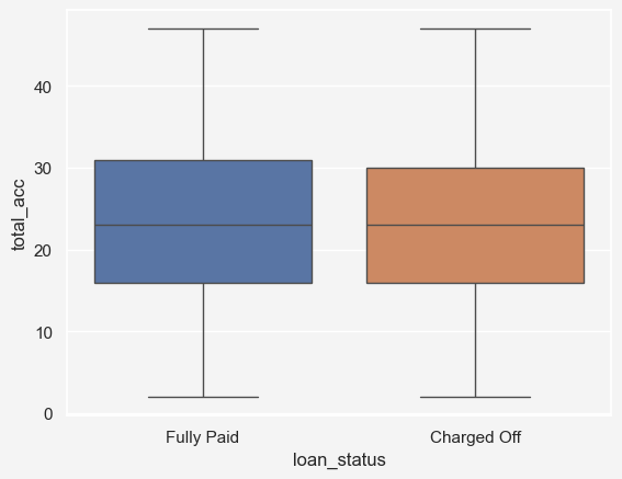
Insights: Number of credit account seems normally distributed among both groups except for some outliers. However, the mean number of credit accounts are slightly higher for the charged off category than the fully paid category. So, higher credit account has some sort of relation with loan being charged off. Also, people who doesn’t have any public record seems to have higher chance of loan status being charged off
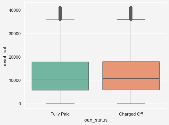
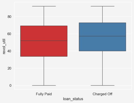
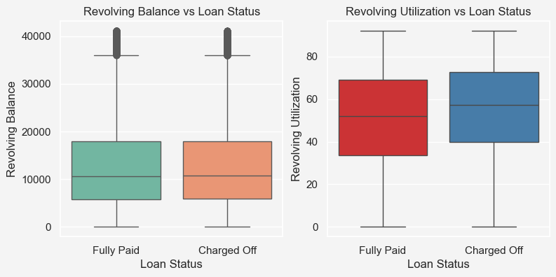
= loandata['revol_bal' ].quantile(0.95 )= loandata[loandata['revol_bal' ] <= revol_bal_threshold]= 'loan_status' , y= 'revol_bal' ,= filtered_revol_bal, hue= 'loan_status' ,= 'Set2'
= loandata['revol_util' ].quantile(0.95 )= loandata[loandata['revol_util' ] <= revol_util_threshold]= 'loan_status' , y= 'revol_util' ,= 'loan_status' , data= filtered_revol_util,= 'Set1'
= plt.figure(figsize= (9 , 4 ))= fig.add_subplot(121 )= loandata['revol_bal' ].quantile(0.95 )= loandata[loandata['revol_bal' ] <= revol_bal_threshold]= 'loan_status' , y= 'revol_bal' ,= filtered_revol_bal, hue= 'loan_status' ,= 'Set2' , ax= ax1'Loan Status' )'Revolving Balance' )'Revolving Balance vs Loan Status' )= fig.add_subplot(122 )= loandata['revol_util' ].quantile(0.95 )= loandata[loandata['revol_util' ] <= revol_util_threshold]= 'loan_status' , y= 'revol_util' ,= 'loan_status' , data= filtered_revol_util,= 'Set1' , ax= ax2'Loan Status' )'Revolving Utilization' )'Revolving Utilization vs Loan Status' )
Text(0.5, 1.0, 'Revolving Utilization vs Loan Status')
'total_acc' ].value_counts()
total_acc
21     14274
22     14255
20     14220
23     13915
24     13874
       ...
151        1
104        1
135        1
108        1
115        1
Name: count, Length: 118, dtype: int64
= plt.figure(figsize= (9 , 4 ))= fig.add_subplot(121 )= loandata['total_acc' ].quantile(0.95 )= loandata[loandata['total_acc' ]<= filtered_total_account_threshold]'loan_status' ] == 'Fully Paid' ]['total_acc' ].hist(= 0.5 , color= 'green' , bins= 30 , label= 'Fully Paid' , ax= ax1'loan_status' ] == 'Charged Off' ]['total_acc' ].hist(= 0.5 , color= 'red' , bins= 30 , label= 'Charged Off' , ax= ax1'Number of Total Credit Acc.' )'Number of Total credit accounts and Loan Status' )= fig.add_subplot(122 )= 'initial_list_status' , hue= 'loan_status' ,= loandata, palette= 'winter' 'Initial Status and Loan Status' )'Initial Status (Funded or Withdrawn)' )
Text(0.5, 0, 'Initial Status (Funded or Withdrawn)')
= 'total_acc' , x= 'loan_status' ,= 'loan_status' ,= filtered_total_account
'application_type' ].value_counts()
application_type
INDIVIDUAL    395189
JOINT            425
DIRECT_PAY       286
Name: count, dtype: int64
'mort_acc' ].value_counts()
mort_acc
0.0     139727
1.0      60392
2.0      49931
3.0      38040
4.0      27880
5.0      18188
6.0      11067
7.0       6050
8.0       3121
9.0       1655
10.0       865
11.0       479
12.0       264
13.0       146
14.0       107
15.0        61
16.0        37
17.0        22
18.0        18
19.0        15
20.0        13
24.0        10
22.0         7
25.0         4
21.0         4
27.0         3
23.0         2
31.0         2
32.0         2
26.0         2
34.0         1
30.0         1
28.0         1
Name: count, dtype: int64
= loandata.groupby('loan_status' )['mort_acc' ].describe()print (mort_acc_summary)
                count      mean       std  min  25%  50%  75%   max
loan_status
Charged Off   72103.0  1.501214  1.974335  0.0  0.0  1.0  2.0  23.0
Fully Paid   286014.0  1.892967  2.182550  0.0  0.0  1.0  3.0  34.0
# Bin the mort_acc column into categories 'mort_acc_group' ] = pd.cut('mort_acc' ], bins= [- 1 , 0 , 2 , 5 , 10 , loandata['mort_acc' ].max ()],= ['0' , '1-2' , '3-5' , '6-10' , '10+' ]# Plot the grouped bar chart = loandata.groupby('mort_acc_group' , 'loan_status' ], observed= False = 'bar' , stacked= False ,= (10 , 6 ), colormap= 'viridis' )'Loan Status by Number of Mortgage Accounts' )'Number of Mortgage Accounts (Grouped)' )'Number of Loans' )= 0 )= 'Loan Status' )
'pub_rec_bankruptcies' ].value_counts()
pub_rec_bankruptcies
0.0    350265
1.0     42776
2.0      1846
3.0       351
4.0        82
5.0        32
6.0         7
7.0         4
8.0         2
Name: count, dtype: int64
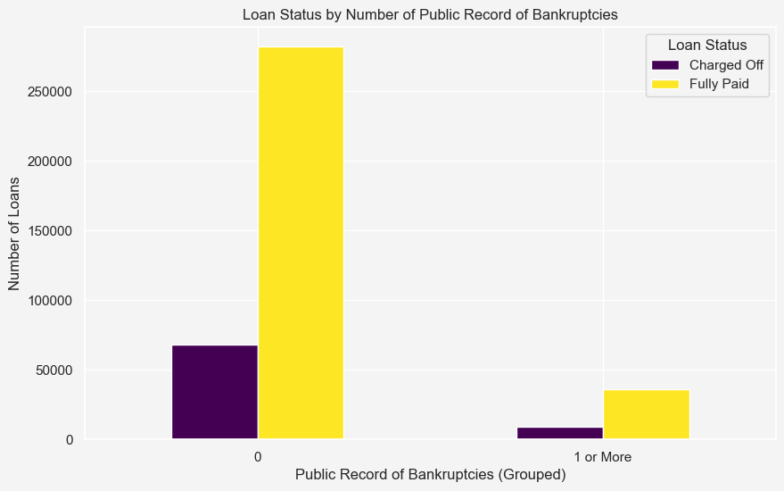
'pub_rec_bankruptcies_group' ] = pd.cut('pub_rec_bankruptcies' ], bins= [- 1 , 0 ,'pub_rec_bankruptcies' ].max ()],= ['0' , '1 or More' ]# Plot the grouped bar chart = loandata.groupby('pub_rec_bankruptcies_group' , 'loan_status' ], observed= False = 'bar' , stacked= False , figsize= (10 , 6 ), colormap= 'viridis' )'Loan Status by Number of Public Record of Bankruptcies' )'Public Record of Bankruptcies (Grouped)' )'Number of Loans' )= 0 )= 'Loan Status' )
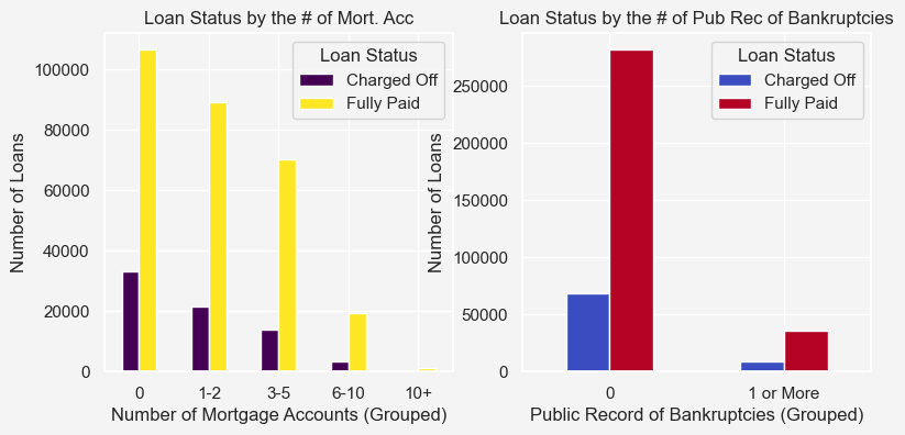
= plt.figure(figsize= (9 , 4 ))= fig.add_subplot(121 )'mort_acc_group' ] = pd.cut('mort_acc' ], bins= [- 1 , 0 , 2 , 5 , 10 , loandata['mort_acc' ].max ()],= ['0' , '1-2' , '3-5' , '6-10' , '10+' ]= loandata.groupby('mort_acc_group' , 'loan_status' ], observed= False = 'bar' , stacked= False ,= 'viridis' , ax= ax1'Loan Status by the # of Mort. Acc' )'Number of Mortgage Accounts (Grouped)' )'Number of Loans' )= 0 )= 'Loan Status' )= fig.add_subplot(122 )'pub_rec_bankruptcies_group' ] = pd.cut('pub_rec_bankruptcies' ], bins= [- 1 , 0 ,'pub_rec_bankruptcies' ].max ()],= ['0' , '1 or More' ]# Plot the grouped bar chart = loandata.groupby('pub_rec_bankruptcies_group' , 'loan_status' ], observed= False = 'bar' , stacked= False ,= 'coolwarm' , ax= ax2'Loan Status by the # of Pub Rec of Bankruptcies' )'Public Record of Bankruptcies (Grouped)' )'Number of Loans' )= 0 )= 'Loan Status' )
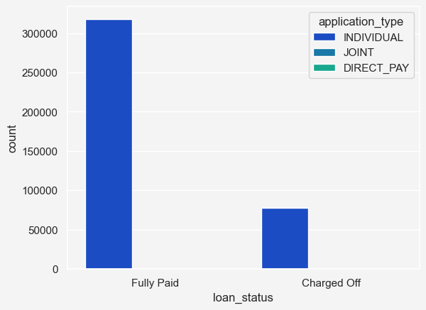
'application_type' ].value_counts()
application_type
INDIVIDUAL    395189
JOINT            425
DIRECT_PAY       286
Name: count, dtype: int64
= 'loan_status' , hue= 'application_type' , = loandata, palette= 'winter'
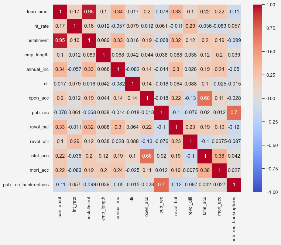
= loandata.select_dtypes(include= ['float64' ,'int64' ])= (10 ,8 ))= True , cmap= 'coolwarm' , vmin=- 1 , vmax= 1 )